Accelerating Stream Processing in Production

Stream processing has become foundational to modern data architectures, enabling organizations to derive real-time insights from continuous data flows. Apache Flink has emerged as the de facto standard for stateful stream processing, offering exactly-once guarantees, low-latency execution, and advanced state management.

However, scaling stream processing from proof-of-concept to production introduces significant challenges. State backends become bottlenecks, access to reference data introduces latency, and the gap between real-time streaming and batch analytics creates data freshness inconsistencies. Organizations that fail to address these blockers often struggle to meet latency requirements or see their pipelines fail to scale gracefully under increasing data volumes.

This article explores three architectural pressure points in production stream processing:

Stateful scaling: Managing state that grows to terabytes
Streaming-lakehouse integration: Bridging real-time and analytical systems
Object storage latency: Accelerating access to reference data

We examine how RocksDB, Apache Fluss, and distributed caching layers address these challenges, providing both architectural guidance and practical configuration examples for production deployments.

1. Blockers for Implementing Stream Processing at Scale
2. RocksDB and State Management in Apache Flink
3. Apache Fluss: Streaming Lakehouse Architecture
4. Accelerating Object Storage Access
Architectural Decision Matrix
6. Conclusion and Future Outlook

1. Blockers for Implementing Stream Processing at Scale

Implementing stream processing in a development or testing environment is fundamentally different from deploying it at production scale. Organizations transitioning from batch processing or proof-of-concept streaming applications often encounter a series of interconnected challenges that can delay or derail production deployments.

1.1 State Management Complexity

State management represents one of the most significant challenges in production stream processing. Stateful stream processing applications must maintain information across event processing cycles. This state can range from simple counters and aggregations to complex windowed computations and join operations.

As applications scale, the state size can grow to terabytes, introducing challenges in:

Storage: Where to persist the state efficiently
Access latency: How to retrieve state quickly for processing
Fault tolerance: How to recover state after failures
Checkpointing: How to snapshot state without blocking processing

The choice of state backend directly impacts checkpoint duration, recovery time, and overall application throughput. The operational complexity of managing large state includes state migration during schema changes, the impact of state size on job rescaling operations, and careful tuning of checkpoint configurations.

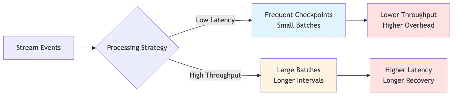
1.2 Latency and Throughput Trade-offs

Stream processing systems must balance latency and throughput requirements, which often conflict. Low-latency processing requires:

Frequent checkpointing
Smaller batch sizes
More frequent state access

But this approach can reduce overall throughput and increase overhead on the state backend.

Conversely, optimizing for throughput by increasing batch sizes and checkpoint intervals introduces:

Higher latency
Larger recovery windows
Greater potential data loss

In production environments, this trade-off becomes particularly acute when serving real-time dashboards or alerting systems that require sub-second data freshness while processing millions of events per second.

1.3 Data Access Patterns and External Lookups

Many stream processing applications require enrichment with reference data or joining with slowly changing dimension tables. This necessitates frequent lookups against external data stores, which can become a significant source of latency.

Object storage systems like Amazon S3, while cost-effective and scalable, introduce access latencies that can be prohibitive for real-time processing. Organizations must implement caching strategies, but caching introduces its own challenges:

Cache invalidation: Ensuring stale data is removed
Consistency: Maintaining accuracy across distributed caches
Memory management: Balancing cache size with available resources

The complexity multiplies when reference data changes frequently, requiring cache updates without disrupting ongoing stream processing.

1.4 Operational Complexity and Expertise Gap

Stream processing systems require specialized operational expertise that is often scarce in the job market. Configuring Flink clusters for optimal performance requires understanding:

Memory models and allocation
Network configurations
State backend tuning
Garbage collection patterns

Troubleshooting production issues demands knowledge of:

Checkpointing mechanisms
Backpressure behavior
Task scheduling
Watermark propagation

The expertise gap is particularly pronounced when organizations transition from managed services to self-hosted deployments, where they must assume responsibility for cluster management, monitoring, and incident response. Many teams discover that the total cost of ownership for stream processing infrastructure extends far beyond hardware and licensing costs.

2. RocksDB and State Management in Apache Flink

Apache Flink provides two primary production state backends for managing application state:

HashMapStateBackend: Stores state in the JVM heap (suitable for small state)
EmbeddedRocksDBStateBackend: Uses an embedded key-value store that persists to local disk, enabling state sizes that far exceed available memory

Note: In Flink versions prior to 1.15, these were called FsStateBackend and RocksDBStateBackend respectively. The naming changed but the underlying concepts remain the same.

Understanding RocksDB's role in Flink's state management is critical for designing and operating production-grade stream processing applications.

2.1 What is RocksDB?

RocksDB is an embeddable persistent key-value store developed at Facebook, based on Google's LevelDB. It is designed for fast storage (SSDs) and provides efficient storage and retrieval of key-value pairs.

Key characteristics:

Embedded library: Runs within the application process, not a separate cluster
LSM-tree structure: Optimized for write-heavy workloads
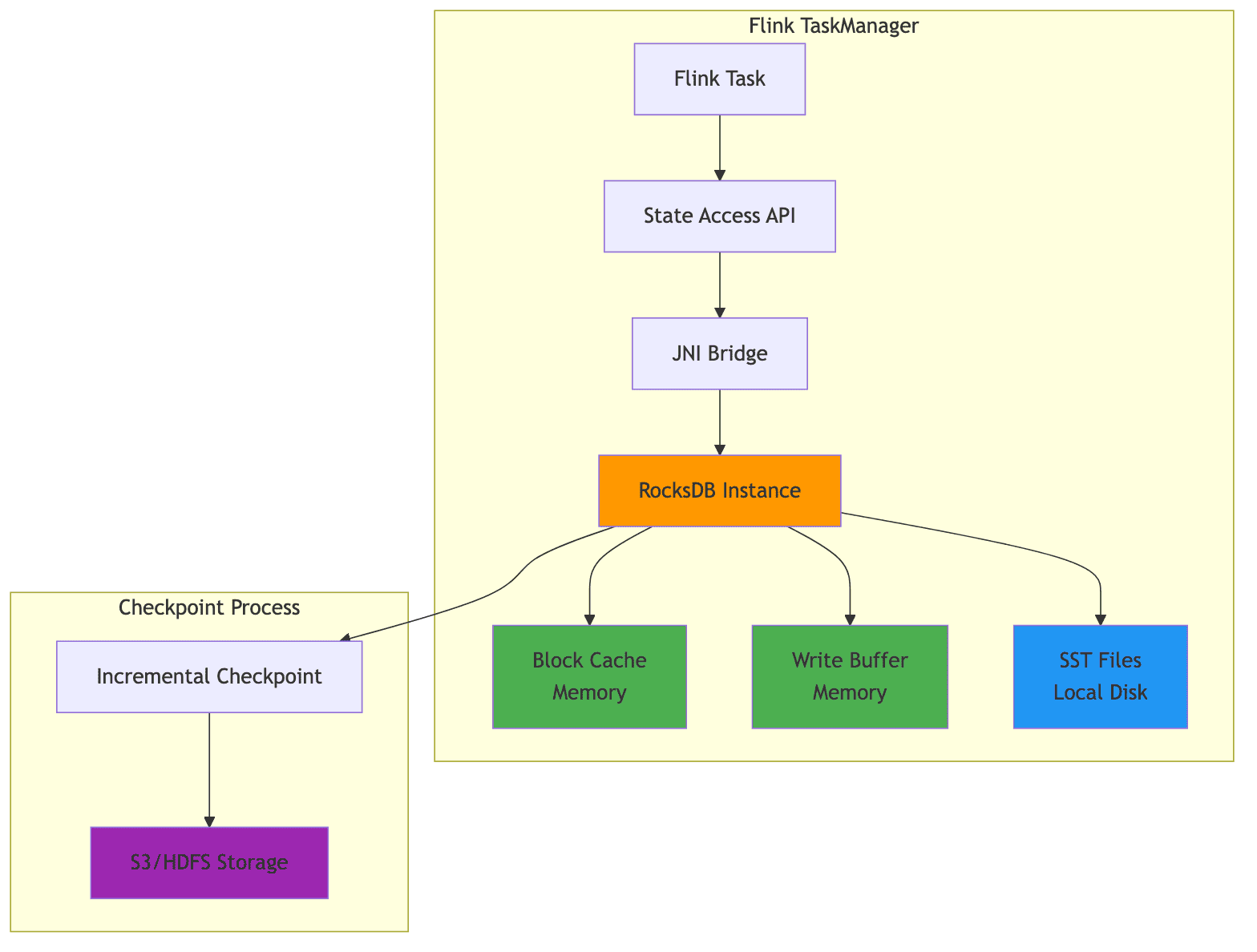
JNI integration: Flink communicates with RocksDB through Java Native Interface
Disk-based working state: Stores working state on local disk with memory caching
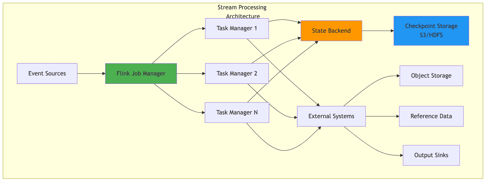
Distributed checkpoint storage: Checkpoints are stored in distributed file systems (S3, HDFS, etc.)

Unlike distributed databases that require separate cluster management, RocksDB runs as a library embedded within the application process. In Flink, RocksDB is embedded in TaskManager processes and interacts with the JVM through the Java Native Interface (JNI).

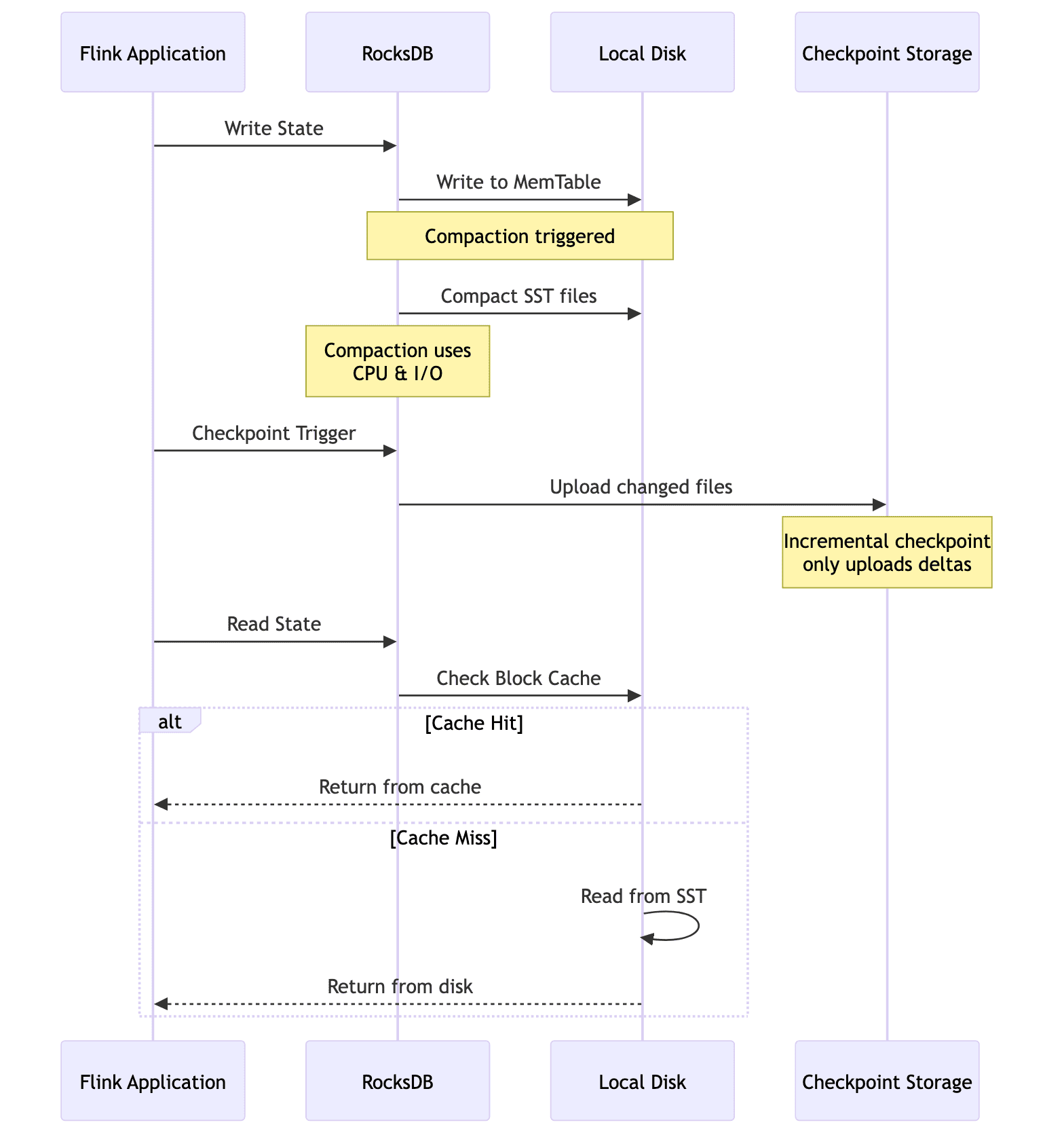
When using EmbeddedRocksDBStateBackend, the working state resides on local disk, but checkpoints (snapshots of state) are stored in distributed storage like S3 or HDFS. Incremental checkpoints only upload the changed SST file deltas, significantly reducing checkpoint overhead for large states.

2.2 When to Use EmbeddedRocksDBStateBackend

The EmbeddedRocksDBStateBackend is the appropriate choice when:

Large state sizes: Application state exceeds what can reasonably fit in JVM heap memory
Long window durations: Applications maintain extensive historical context
Complex keyed state: Applications with large keyed state requirements
Incremental checkpointing: Need for reduced checkpoint duration

Since RocksDB stores state off-heap and on disk, it provides more predictable latency by avoiding the impact of garbage collection pauses that can affect heap-based state backends. However, this comes at the cost of higher per-access latency due to serialization overhead and disk I/O.

Comparison of State Backends:

Feature	HashMapStateBackend	EmbeddedRocksDBStateBackend
State Location	JVM Heap	Off-heap (RocksDB on disk)
Checkpoint Storage	Distributed FS	Distributed FS
State Size Limit	Limited by heap	Limited by disk
Access Latency	Lowest	Higher (serialization + disk I/O)
GC Impact	High	Low
Incremental Checkpoints	No	Yes
Production Ready	Yes (small to medium state)	Yes (large state)
Best For	State < few GB	State > tens of GB

2.3 State Management Problems at Scale

As state sizes grow into the terabyte range, organizations encounter several challenges with RocksDB-based state management:

1. Checkpoint Duration
Even with incremental checkpointing enabled, large checkpoints consume network bandwidth and storage I/O, potentially impacting the performance of other operations. Checkpoint duration directly affects the Recovery Point Objective (RPO) of your streaming application.

2. Recovery Time
Recovery time after failures increases with state size, as the application must restore state from the checkpoint location. This recovery time can violate service level agreements for mission-critical applications. For very large states, recovery can take hours.

3. Rescaling Operations
When the parallelism of a job is changed, state must be redistributed across TaskManagers. This can take hours for very large states and requires careful planning to minimize downtime.

4. Background Operations
Background operations in RocksDB, such as compaction and flushing, can interfere with stream processing performance. When RocksDB compacts files in the background, it consumes CPU and I/O resources that would otherwise be available for event processing, causing unpredictable latency spikes. This is especially visible under write-heavy workloads with high key cardinality, where many SST files are generated and require frequent compaction.

5. Memory Management
Each column family in RocksDB maintains its own block cache and write buffers. Improper configuration can lead to excessive memory usage or suboptimal cache hit rates.

2.4 Configuration Best Practices

Configuring RocksDB for production workloads requires attention to several key parameters:

1. Local Storage Configuration
The local directory for RocksDB files should be on high-performance local storage, ideally SSDs, rather than network-attached storage.

2. Memory Management
Flink's managed memory system (introduced in Flink 1.10) automatically allocates memory for RocksDB. For fine-grained control, you can disable managed memory and configure block cache and write buffer sizes explicitly.

3. Background Threads
The number of background threads should be increased from the default for machines with many CPU cores, as this parallelizes compaction and flushing operations.

4. Bloom Filters
For applications with frequent read operations, enabling bloom filters can significantly reduce disk reads by quickly determining whether a key might exist in a file.

Configuration Example (flink-conf.yaml):

1# Enable RocksDB state backend with incremental checkpointing
2state.backend.type: rocksdb
3state.backend.incremental: true
4state.checkpoints.dir: s3://your-bucket/flink-checkpoints
5
6# RocksDB local directory on high-performance SSD
7state.backend.rocksdb.localdir: /mnt/ssd/rocksdb
8
9# Enable managed memory for RocksDB
10state.backend.rocksdb.memory.managed: true
11
12# Enable predefined options for better performance
13state.backend.rocksdb.predefined-options: SPINNING_DISK_OPTIMIZED_HIGH_MEM
14
15# Write buffer configuration
16state.backend.rocksdb.writebuffer.size: 64mb
17state.backend.rocksdb.writebuffer.count: 4
18
19# Block cache size (if not using managed memory)
20state.backend.rocksdb.block.cache-size: 256mb
21
22# Checkpoint configuration
23execution.checkpointing.interval: 5min
24execution.checkpointing.mode: EXACTLY_ONCE
25execution.checkpointing.timeout: 10min
26

Note: Some configuration keys vary by Flink version. For fine-grained control over RocksDB behavior (such as background thread tuning), use RocksDBOptionsFactory for programmatic configuration.

Programmatic Configuration:

1// Configure RocksDB state backend programmatically
2EmbeddedRocksDBStateBackend backend = new EmbeddedRocksDBStateBackend(true);
3
4// Set local directory
5backend.setDbStoragePath("/mnt/ssd/rocksdb");
6
7// Configure predefined options
8backend.setPredefinedOptions(PredefinedOptions.SPINNING_DISK_OPTIMIZED_HIGH_MEM);
9
10// Set custom RocksDB options
11backend.setRocksDBOptions(new RocksDBOptionsFactory() {
12    @Override
13    public DBOptions createDBOptions(DBOptions currentOptions, Collection<AutoCloseable> handlesToClose) {
14        return currentOptions
15            .setMaxBackgroundJobs(8)
16            .setMaxOpenFiles(-1)
17            .setStatsDumpPeriodSec(0);
18    }
19    
20    @Override
21    public ColumnFamilyOptions createColumnOptions(ColumnFamilyOptions currentOptions, Collection<AutoCloseable> handlesToClose) {
22        return currentOptions
23            .setTableFormatConfig(
24                new BlockBasedTableConfig()
25                    .setBlockSize(128 * 1024)
26                    .setBlockCacheSize(256 * 1024 * 1024)
27                    .setFilterPolicy(new BloomFilter(10, false))
28            )
29            .setWriteBufferSize(64 * 1024 * 1024)
30            .setMaxWriteBufferNumber(4);
31    }
32});
33
34// Note: setStateBackend() is deprecated in Flink 1.15+
35// Prefer using configuration file or StreamExecutionEnvironment.configure()
36env.setStateBackend(backend);
37

3. Apache Fluss: Streaming Lakehouse Architecture

Apache Fluss (currently incubating) represents a significant evolution in the stream processing landscape by addressing the fundamental tension between real-time streaming and analytical lakehouse architectures.

Traditional lakehouse formats like Apache Iceberg, Apache Hudi, and Delta Lake excel at providing ACID transactions, schema evolution, and efficient analytical queries on data lakes. However, they struggle to provide sub-second data freshness due to the inherent trade-off between write frequency and read efficiency. Frequent writes create many small files that are inefficient for queries, while batching writes for efficiency increases latency.

Important Note: Fluss is not a replacement for Kafka in all cases. While Kafka is a distributed log for high-throughput pub-sub messaging, Fluss combines log semantics with lakehouse semantics, making it ideal for scenarios where you need both real-time streaming and immediate analytical access to the same data. For pure streaming use cases without analytical requirements, Kafka remains the simpler choice.

3.1 The Streaming Lakehouse Concept

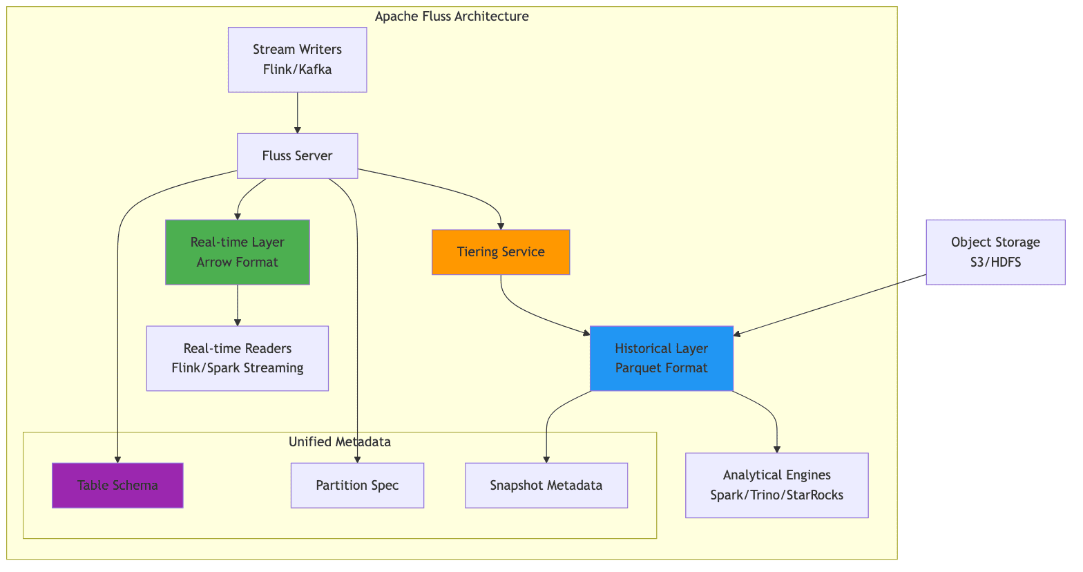
Fluss introduces the concept of a "Streaming Lakehouse" that unifies real-time streaming data with historical lakehouse data. It achieves this by maintaining two complementary data layers:

Real-time Layer: Stores data in streaming-optimized Arrow format for sub-second access
Historical Layer: Stores compacted data in Parquet format for efficient analytical queries

A tiering service continuously compacts data from the real-time layer to the historical layer, maintaining consistency between both representations. This architecture allows applications to access truly real-time data through the streaming layer while benefiting from the query efficiency and cost-effectiveness of the lakehouse format for historical analysis.

3.2 Key Features and Benefits

Fluss provides several key features that address common challenges in stream processing architectures:

1. Unified Metadata
Fluss allows users to manage a single table definition that encompasses both real-time and historical data. This eliminates the complexity of maintaining separate streaming and batch tables with synchronized schemas.

2. Union Reads
Queries transparently combine data from both the real-time and historical layers, providing a complete view without requiring users to understand the underlying data organization.

1-- Query automatically combines real-time and historical data
2SELECT customer_id, SUM(amount) as total_spend
3FROM fluss_catalog.ecommerce.orders
4WHERE order_date >= '2026-01-01'
5GROUP BY customer_id;
6

3. Low-Latency Writes
Flink applications can write to Fluss with low latency, similar to writing to Kafka, while simultaneously providing lakehouse access to the same data.

4. Multiple Lakehouse Formats
Fluss currently supports Apache Paimon, Apache Iceberg, and Lance as lakehouse storage formats, providing flexibility in choosing the appropriate format for specific use cases.

5. Automatic Tiering
The tiering service automatically manages the lifecycle of data, moving it from the real-time layer to the historical layer based on configurable policies.

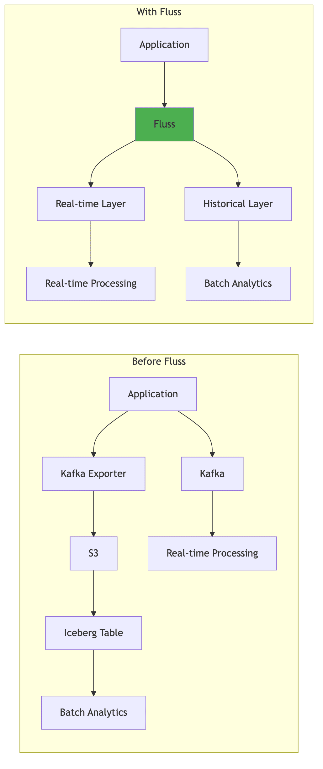
Architecture Comparison:

Traditional Approach	With Fluss
Separate Kafka + Data Lake	Unified streaming storage
Dual ingestion pipelines	Single write path
Minutes to hours latency	Sub-second latency
Schema sync complexity	Unified schema management
Separate metadata	Single metadata layer

3.3 Appropriate Use Cases

Fluss is particularly well-suited for:

1. Real-time Operational Analytics
E-commerce platforms that need real-time inventory dashboards alongside historical sales analysis represent a prime use case. The real-time layer provides up-to-the-second inventory levels, while the historical layer enables trend analysis and forecasting.

2. Financial Services
Financial institutions requiring real-time fraud detection with the ability to perform historical pattern analysis benefit significantly from Fluss's architecture. The real-time layer powers fraud detection models, while the historical layer enables compliance reporting and forensic analysis.

3. Simplified Architecture
Organizations currently maintaining separate Kafka topics for streaming and batch exports to data lakes can simplify their architecture by adopting Fluss as a unified streaming storage layer.

4. IoT and Sensor Data
IoT applications that need to react to sensor data in real-time while maintaining long-term historical data for analysis and machine learning model training.

When Not to Use Fluss:

For applications that only require either pure streaming or pure batch processing, the additional complexity of Fluss may not be justified. Additionally, organizations without the operational expertise to manage a new storage system should carefully evaluate the trade-offs.

4. Accelerating Object Storage Access

Object storage systems such as Amazon S3, Google Cloud Storage, and Azure Blob Storage have become the default choice for storing large volumes of data due to their scalability, durability, and cost-effectiveness. However, their access latency, particularly for random read patterns, can be problematic for stream processing workloads that require low-latency access to reference data or dimension tables.

Caching layers address this challenge by providing a high-performance buffer between compute engines and object storage. There are two architectural approaches to accelerating object storage access:

File-level acceleration: Transparent caching of files and objects (e.g., Alluxio)
Data-level acceleration: Materialized key-value or SQL grids that pre-load data into memory (e.g., Apache Ignite)

The choice between these approaches depends on your access patterns, consistency requirements, and operational constraints.

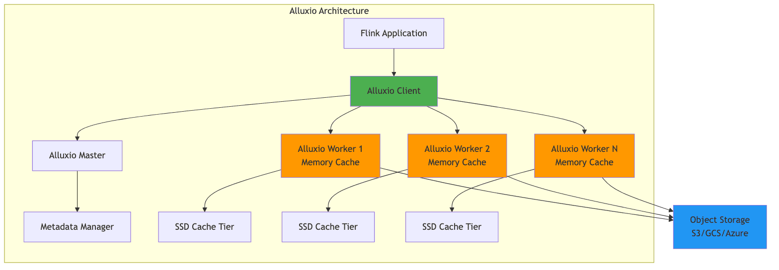
4.1 Alluxio: Distributed Data Orchestration

Alluxio is a distributed caching layer that sits between compute frameworks and storage systems, providing data orchestration and acceleration. It presents a unified namespace that can mount multiple underlying storage systems, transparently caching frequently accessed data in memory or on local SSDs.

Key Benefits for Stream Processing:

Reduced Latency: Cache dimension tables and reference data that are frequently accessed during join operations
Higher Throughput: Serve data from local cache instead of making repeated calls to object storage
Cost Savings: Reduced API calls to object storage can translate to significant cost savings at scale
Write Caching: Alluxio AI 3.8 introduced write caching, addressing the bottleneck of writing results back to object storage

Use Cases in Stream Processing:

1. Dimension Table Joins with Flink SQL

The most practical way to leverage Alluxio in stream processing is through Flink's SQL API, where entire dimension tables stored as Parquet files are accessed through the Alluxio cache.

1-- Configure Alluxio as the file system (done at cluster level)
2-- Flink jobs access files via alluxio:// protocol
3
4-- Create a dimension table backed by Parquet files in Alluxio
5CREATE TABLE product_dimensions (
6    product_id STRING,
7    product_name STRING,
8    category STRING,
9    price DECIMAL(10, 2)
10) WITH (
11    'connector' = 'filesystem',
12    'path' = 'alluxio://master:19998/dimensions/products',
13    'format' = 'parquet'
14);
15
16-- Kafka source table
17CREATE TABLE order_stream (
18    order_id STRING,
19    product_id STRING,
20    quantity INT,
21    order_time TIMESTAMP(3)
22) WITH (
23    'connector' = 'kafka',
24    'topic' = 'orders',
25    'properties.bootstrap.servers' = 'kafka:9092',
26    'format' = 'json'
27);
28
29-- Join streaming orders with cached dimension table
30-- Alluxio transparently caches the Parquet files for fast repeated access
31SELECT 
32    o.order_id,
33    o.product_id,
34    p.product_name,
35    p.category,
36    o.quantity,
37    o.quantity * p.price as order_value
38FROM order_stream o
39LEFT JOIN product_dimensions FOR SYSTEM_TIME AS OF o.order_time AS p
40ON o.product_id = p.product_id;
41

2. Broadcast State with Alluxio-Cached Data

For DataStream API, load dimension data from Alluxio-cached files into broadcast state:

1// Alluxio is configured at cluster level via flink-conf.yaml
2// alluxio.master.hostname=master
3// alluxio.master.port=19998
4
5// Read dimension data from Alluxio path
6// The files are transparently cached by Alluxio
7FileSource<Product> dimensionSource = FileSource
8    .forRecordStreamFormat(new ParquetReaderFactory<>(), 
9        new Path("alluxio://master:19998/dimensions/products.parquet"))
10    .build();
11
12// Load into broadcast state for enrichment
13MapStateDescriptor<String, Product> dimensionStateDesc = 
14    new MapStateDescriptor<>("dimensions", String.class, Product.class);
15
16BroadcastStream<Product> dimensionBroadcast = env
17    .fromSource(dimensionSource, WatermarkStrategy.noWatermarks(), "Dimensions")
18    .broadcast(dimensionStateDesc);
19
20// Main event stream
21DataStream<Order> orders = env.addSource(new KafkaSource<>(...));
22
23// Enrich orders with broadcast dimension data
24DataStream<EnrichedOrder> enriched = orders
25    .connect(dimensionBroadcast)
26    .process(new BroadcastProcessFunction<Order, Product, EnrichedOrder>() {
27        @Override
28        public void processElement(Order order, 
29                                   ReadOnlyContext ctx, 
30                                   Collector<EnrichedOrder> out) {
31            ReadOnlyBroadcastState<String, Product> state = 
32                ctx.getBroadcastState(dimensionStateDesc);
33            Product product = state.get(order.getProductId());
34            out.collect(new EnrichedOrder(order, product));
35        }
36        
37        @Override
38        public void processBroadcastElement(Product product, 
39                                           Context ctx, 
40                                           Collector<EnrichedOrder> out) {
41            ctx.getBroadcastState(dimensionStateDesc)
42               .put(product.getId(), product);
43        }
44    });
45

Key Points:

Alluxio is configured at the cluster level, not within individual jobs
It provides transparent caching—Flink reads from alluxio:// paths like any file system
Best for scenarios where dimension data is read repeatedly by multiple jobs
Reduces S3 API calls and improves read throughput for frequently accessed files

Configuration:

1# Alluxio configuration for stream processing
2alluxio.user.file.cache.enabled=true
3alluxio.user.file.readtype.default=CACHE
4alluxio.user.file.writetype.default=CACHE_THROUGH
5
6# Memory allocation
7alluxio.worker.memory.size=32GB
8alluxio.worker.tieredstore.levels=2
9alluxio.worker.tieredstore.level0.alias=MEM
10alluxio.worker.tieredstore.level0.dirs.path=/mnt/ramdisk
11alluxio.worker.tieredstore.level1.alias=SSD
12alluxio.worker.tieredstore.level1.dirs.path=/mnt/ssd
13

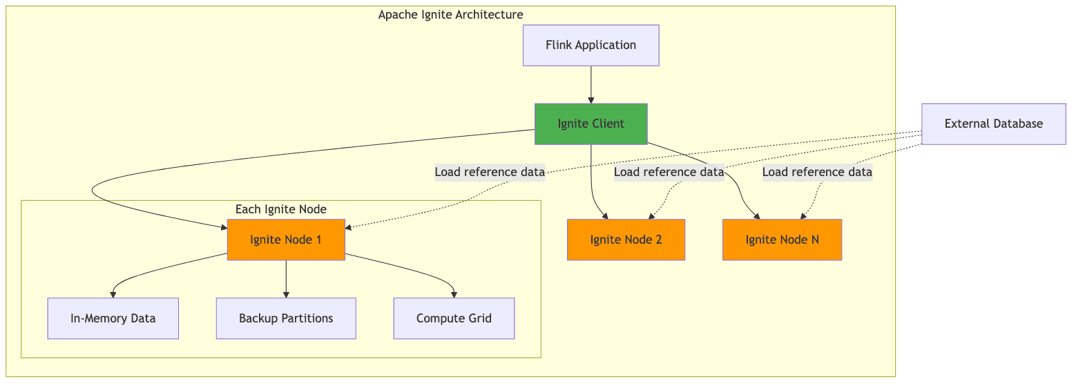
4.2 Apache Ignite: In-Memory Data Grid

Apache Ignite provides a different approach to data acceleration through its in-memory data grid capabilities. Unlike Alluxio, which focuses on file-based caching, Ignite provides a distributed key-value store that can be used directly for caching reference data.

Key Features:

Sub-millisecond Access: Cached data with sub-millisecond access times
SQL Capabilities: Query cached data using standard SQL syntax
Distributed Transactions: ACID transactions across the data grid
Compute Co-location: Run computations where data is cached

Use Cases in Stream Processing:

1. Real-time Lookups

1// Flink enrichment with Ignite cache
2public class IgniteEnrichmentFunction extends RichMapFunction<Event, EnrichedEvent> {
3    private static transient Ignite ignite; // Static to share across instances
4    private transient IgniteCache<String, Customer> customerCache;
5    
6    @Override
7    public void open(Configuration parameters) {
8        // Use singleton pattern to avoid multiple Ignite client instances
9        if (ignite == null) {
10            synchronized (IgniteEnrichmentFunction.class) {
11                if (ignite == null) {
12                    IgniteConfiguration cfg = new IgniteConfiguration();
13                    cfg.setClientMode(true);
14                    cfg.setIgniteInstanceName("flink-ignite-client");
15                    ignite = Ignition.start(cfg);
16                }
17            }
18        }
19        customerCache = ignite.cache("customers");
20    }
21    
22    @Override
23    public EnrichedEvent map(Event event) {
24        // Sub-millisecond lookup
25        Customer customer = customerCache.get(event.getCustomerId());
26        return new EnrichedEvent(event, customer);
27    }
28    
29    @Override
30    public void close() {
31        // Don't close static Ignite instance
32        // It will be shared across all operator instances
33    }
34}
35

2. Distributed Counters with Proper Atomicity

1// Use Ignite's distributed atomic types for shared aggregation state
2public class SharedStateAggregation extends RichFlatMapFunction<Event, Aggregation> {
3    private static transient Ignite ignite;
4    
5    @Override
6    public void open(Configuration parameters) {
7        if (ignite == null) {
8            synchronized (SharedStateAggregation.class) {
9                if (ignite == null) {
10                    IgniteConfiguration cfg = new IgniteConfiguration();
11                    cfg.setClientMode(true);
12                    ignite = Ignition.start(cfg);
13                }
14            }
15        }
16    }
17    
18    @Override
19    public void flatMap(Event event, Collector<Aggregation> out) {
20        String key = event.getAggregationKey();
21        
22        // Use IgniteAtomicLong for distributed atomic operations
23        // This ensures thread-safe distributed increments
24        IgniteAtomicLong counter = ignite.atomicLong(
25            key,           // counter name
26            0,             // initial value
27            true           // create if not exists
28        );
29        
30        long newValue = counter.incrementAndGet();
31        out.collect(new Aggregation(key, newValue));
32    }
33}
34

3. Cache Loading from CDC Stream

1// Keep Ignite cache in sync with source database using CDC
2DataStream<ChangeEvent> cdcStream = env.addSource(new DebeziumSource<>(...));
3
4cdcStream.addSink(new RichSinkFunction<ChangeEvent>() {
5    private static transient Ignite ignite;
6    private transient IgniteCache<String, Customer> cache;
7    
8    @Override
9    public void open(Configuration parameters) {
10        if (ignite == null) {
11            synchronized (this.getClass()) {
12                if (ignite == null) {
13                    ignite = Ignition.start(new IgniteConfiguration().setClientMode(true));
14                }
15            }
16        }
17        cache = ignite.cache("customers");
18    }
19    
20    @Override
21    public void invoke(ChangeEvent event, Context context) {
22        switch (event.getOperation()) {
23            case INSERT:
24            case UPDATE:
25                cache.put(event.getKey(), event.getValue());
26                break;
27            case DELETE:
28                cache.remove(event.getKey());
29                break;
30        }
31    }
32});
33

Key Points:

Use static singleton pattern for Ignite client to avoid creating multiple instances per operator
Use IgniteAtomicLong for distributed atomic operations, not Java's AtomicLong
Ignite provides strong consistency guarantees for cache operations
Best for key-value lookups with frequent updates (e.g., dimension tables, aggregation state)

Comparison: Alluxio vs Apache Ignite

Feature	Alluxio	Apache Ignite
Primary Use Case	File-based caching	Key-value caching
Data Model	Files/Objects	Key-value, SQL
Access Pattern	File I/O	Get/Put, SQL queries
Best For	Parquet/Avro files	Dimension tables
Latency	Low (cached files)	Very low (in-memory)
Query Support	Via mounted engines	Native SQL
Consistency Model	Transparent caching	Strong consistency
Write Support	Cache-through	Direct writes

4.3 Implementation Considerations

Implementing caching layers requires careful consideration of several factors:

1. Consistency and Invalidation

Stream processing applications often require access to the latest version of reference data. Cache invalidation strategies must ensure that stale data is either evicted or updated when the source data changes.

Alluxio TTL-based Invalidation:

1# Set TTL for cached dimension tables
2alluxio.user.file.metadata.sync.interval=5min
3alluxio.user.file.passive.cache.enabled=true
4

Ignite Change Data Capture:

1// Update Ignite cache from CDC stream
2DataStream<ChangeEvent> cdcStream = env.addSource(new DebeziumSource<>(...));
3
4cdcStream.addSink(new RichSinkFunction<ChangeEvent>() {
5    private transient IgniteCache<String, Customer> cache;
6    
7    @Override
8    public void open(Configuration parameters) {
9        cache = Ignition.start(config).cache("customers");
10    }
11    
12    @Override
13    public void invoke(ChangeEvent event, Context context) {
14        switch (event.getOperation()) {
15            case INSERT:
16            case UPDATE:
17                cache.put(event.getKey(), event.getValue());
18                break;
19            case DELETE:
20                cache.remove(event.getKey());
21                break;
22        }
23    }
24});
25

2. Resource Management

Caching layers require dedicated memory and potentially SSD storage, which must be provisioned appropriately to avoid impacting the resources available for stream processing itself.

1# Kubernetes deployment with resource allocation
2apiVersion: v1
3kind: Pod
4metadata:
5  name: flink-taskmanager
6spec:
7  containers:
8  - name: taskmanager
9    resources:
10      requests:
11        memory: "8Gi"
12        cpu: "4"
13      limits:
14        memory: "16Gi"
15        cpu: "8"
16  - name: alluxio-worker
17    resources:
18      requests:
19        memory: "32Gi"
20        cpu: "2"
21      limits:
22        memory: "64Gi"
23        cpu: "4"
24

3. Monitoring

Monitoring cache hit rates, eviction rates, and access latency is essential for tuning the caching configuration and justifying the infrastructure investment.

Key Metrics to Monitor:

Cache hit rate
Cache miss rate
Average access latency
Eviction rate
Memory utilization
Network throughput
Object storage API call reduction

1// Expose Alluxio metrics to Prometheus
2MetricRegistry registry = AlluxioWorkerMonitor.getMetricRegistry();
3registry.gauge("cache.hit.rate", () -> 
4    (double) cacheHits / (cacheHits + cacheMisses)
5);
6

4. Production Cost Considerations

Understanding the cost implications of different caching strategies is critical for production deployments:

S3 API Call Costs:

Without caching: If a dimension table is read 1000 times/sec, that's 86.4M GET requests/day
At $0.0004 per 1000 requests =$ 34.56/day or ~$1,000/month just for reads
With Alluxio caching: Reduced to initial load + occasional refreshes = ~$1-2/month

Checkpoint Storage Growth:

RocksDB incremental checkpoints grow metadata over time
Without cleanup, metadata can reach hundreds of GB
Recommendation: Enable checkpoint retention and expired snapshot cleanup
Configure state.checkpoints.num-retained: 3 to limit storage costs

Cache Infrastructure Costs:

Alluxio worker with 64GB RAM + 1TB NVMe SSD: ~$200-300/month per node
Apache Ignite with 128GB RAM: ~$400-500/month per node
ROI calculation: Cache cost vs. S3 API costs + latency improvement value

5. Failure Mode Analysis

Understanding failure modes helps design more resilient systems:

Failure Scenario	Impact	Mitigation
RocksDB local SSD failure	Task failure, restore from checkpoint	Use RAID or redundant disks; fast SSD replacement
Cold cache (Alluxio restart)	Temporary performance degradation	Gradual warm-up; prioritize critical datasets
Ignite node failure	Backup partitions serve requests	Configure backup count ≥ 2
Checkpoint storage unavailable	Cannot create checkpoints; risk of data loss	Use highly available storage (S3, HDFS HA)
Large state backfill	Hours of replay, high resource usage	Pre-warm state; use savepoints for planned restarts

Cold Cache Scenario:
When Alluxio restarts, all cached data is lost. The first access will be slow (S3 latency), but subsequent accesses will benefit from the cache. To minimize impact:

Implement gradual warm-up by pre-loading critical datasets
Use Alluxio's pinning feature for high-priority data
Monitor cache miss rate and alert on sustained high values

Architectural Decision Matrix

Choosing the right technology for your stream processing challenges requires understanding the trade-offs. Here's a decision matrix to guide your architectural choices:

Problem	Solution	Primary Benefit	Key Trade-off	When to Use
Large keyed state (>100GB)	EmbeddedRocksDBStateBackend	Unlimited state size	Higher access latency (serialization)	State exceeds heap memory
Small state (<10GB)	HashMapStateBackend	Lowest latency	Limited by heap size	Fast state access critical
Streaming + batch analytics	Apache Fluss	Unified real-time + historical data	New infrastructure to manage	Need sub-second fresh analytics
S3 lookup latency	Alluxio	Transparent file caching	Additional memory tier required	Repeated file access patterns
Dimension table lookups	Apache Ignite	Sub-millisecond KV access	Consistency management overhead	High-frequency KV lookups
Checkpoint duration	Incremental checkpoints	Only upload deltas	Metadata accumulation	State >100GB
Recovery time	Smaller checkpoints + local state	Faster restore	Less fault tolerance	Low RTO requirements
Schema evolution	Fluss unified metadata	Single schema for stream + batch	Coupled architecture	Frequent schema changes

Decision Tree for State Backend:

1State Size?
2├─ <5GB → HashMapStateBackend
3├─ 5-50GB → Either (benchmark both)
4└─ >50GB → EmbeddedRocksDBStateBackend
5    └─ Enable incremental checkpointing
6

Decision Tree for Caching:

1Access Pattern?
2├─ File-based (Parquet, Avro)
3│   └─ Alluxio
4│       └─ Configure tiered storage (Memory → SSD)
5└─ Key-value lookups
6    ├─ Read-heavy → Ignite (replicated mode)
7    └─ Write-heavy → Ignite (partitioned mode) or external DB
8

Decision Tree for Lakehouse Integration:

1Need sub-second fresh analytics?
2├─ Yes → Consider Fluss
3│   └─ Are you maintaining separate Kafka + Data Lake?
4│       ├─ Yes → Strong candidate for Fluss
5│       └─ No → Evaluate operational overhead
6└─ No → Standard Kafka + batch ingestion to lakehouse
7    └─ Latency tolerance >5 minutes
8

6. Conclusion and Future Outlook

Accelerating stream processing in production environments requires a holistic approach that addresses state management, data access patterns, and the integration between streaming and analytical systems.

Key Takeaways:

State Management: RocksDB remains the state backend of choice for large-state applications in Flink, but organizations must invest in proper configuration and operational expertise to realize its benefits.
Streaming Lakehouse: The emergence of Apache Fluss offers a promising solution to the streaming-lakehouse integration challenge, potentially simplifying architectures that currently require separate systems for real-time and batch processing.
Caching Strategies: Caching layers like Alluxio and Apache Ignite provide practical solutions for accelerating data access from object storage, with the choice between them depending on specific access patterns and consistency requirements.
Operational Excellence: Success in production stream processing requires more than just technical solutions—it demands operational expertise, comprehensive monitoring, and a deep understanding of the trade-offs involved.

Future Trends:

Several trends are likely to shape the evolution of stream processing acceleration:

1. State Disaggregation
Flink 2.0's proposed architecture promises to separate compute from state storage, potentially reducing recovery times and enabling more flexible scaling. This will allow independent scaling of compute and state resources.

2. Unified Streaming Storage
The continued development of Apache Fluss and similar streaming storage systems will likely blur the distinction between streaming and batch processing further, leading to simpler architectures.

3. AI/ML Integration
The integration of AI and machine learning workloads with stream processing pipelines will drive demand for even lower latency and more sophisticated state management capabilities. Real-time feature stores and online model inference will become first-class citizens in stream processing frameworks.

4. Cloud-Native Evolution
Stream processing systems will continue to evolve towards cloud-native architectures, with better Kubernetes integration, serverless deployment options, and automatic scaling based on workload.

5. Hardware Acceleration
As specialized hardware for data processing (GPUs, FPGAs, smart NICs) becomes more accessible, stream processing frameworks will integrate with these accelerators to achieve even lower latencies.

Organizations investing in stream processing infrastructure should monitor these developments and plan for architectural flexibility as the technology landscape continues to evolve. The key is not to chase every new technology, but to understand the fundamental challenges your organization faces and select solutions that address those specific needs.

Accelerating Stream Processing in Production

Accelerating Stream Processing in Production

Contents

1. Blockers for Implementing Stream Processing at Scale

1.1 State Management Complexity

1.2 Latency and Throughput Trade-offs

1.3 Data Access Patterns and External Lookups

1.4 Operational Complexity and Expertise Gap

2. RocksDB and State Management in Apache Flink

2.1 What is RocksDB?

2.2 When to Use EmbeddedRocksDBStateBackend

2.3 State Management Problems at Scale

2.4 Configuration Best Practices

3. Apache Fluss: Streaming Lakehouse Architecture

3.1 The Streaming Lakehouse Concept

3.2 Key Features and Benefits

3.3 Appropriate Use Cases

4. Accelerating Object Storage Access

4.1 Alluxio: Distributed Data Orchestration

4.2 Apache Ignite: In-Memory Data Grid

4.3 Implementation Considerations

Architectural Decision Matrix

6. Conclusion and Future Outlook

Enjoyed this post? Subscribe for more!