Distributed Data Systems: Understanding Join Algorithms

In the world of large-scale data processing, the join operation is the most fundamental, powerful and often performance-critical operation. It's the mechanism through which datasets are unified, relationships are discovered and raw data is transformed into meaningful insights.
This becomes more critical in a distributed environment where data is spread across a cluster of machines. The choice of the join algorithm then is not a minor implementation detail, but a primary determinant of the job's performance, resource consumption and scalability.

For many data engineers, the internal workings of a query engine are mostly opaque. Queries are submitted and results are returned. However, when performance degrades or jobs fail, this opacity becomes a barrier to effective troubleshooting and optimization. The goal of this article is to understand the join strategies employed by distributed query engines like Spark and Trino.

Apache Spark is a general purpose fault-tolerant distributed data processing engine designed for a wide range of workloads. Trino (formerly PrestoSQL) is a high-performance, low-latency federated distributed query engine optimized for interactive queries across diverse data sources.

I personally have more experience with Spark, having used it extensively in production systems. My understanding of Trino is based on documentation, community discussions and some hands-on experimentation. If you spot any inaccuracies or have additional insights, please reach out!

The codebase that demonstrates different join algorithms is available on Github.

🔗 Source Code: abyssnlp/join-algorithms

It contains simple and easy to understand Python implementations of various join algorithms. Feel free to explore the code, run and experiment with how these algorithms work.

---

Here is the entire series so far:

1. Understanding Replication. Part-1
2. Understanding Replication. Part-2
3. Distributed Postgres Architectures
4. Leaderless Replication: Quorums, Hinted Handoff and Read repair
5. Understanding Join Algorithms (You're here)

---

Contents

1. Architectural Context
   1. Apache Spark
      1. Execution Model
      2. Fault Tolerance
   2. Trino
      1. Execution Model
      2. Fault Tolerance
   3. The Impact on Join Strategies
2. Join Execution and Optimization in Apache Spark
   1. Catalyst Optimizer
   2. Tungsten Execution Engine
   3. Join Algorithms in Spark
      1. Broadcast Hash Join (BHJ)
      2. Shuffle Sort-Merge Join (SMJ)
      3. Shuffle Hash Join (SHJ)
3. Join Execution and Optimization in Trino
   1. Join Algorithms in Trino
      1. Partitioned Join
      2. Broadcast Join
      3. Cost-Based Optimizer (CBO)
4. Implementing Join Algorithms in Python
   1. Hash Join
      1. Implementation Details
      2. Time Complexity Analysis
   2. Sort-Merge Join
      1. Implementation Details
      2. External Sort-Merge Join
      3. Time Complexity Analysis
   3. Grace & Parallel Hash Joins
      1. Grace Hash Join
         1. Implementation Details
         2. Hash Function Distribution
         3. Time Complexity Analysis
      2. Parallel Hash Join
         1. Implementation Details
         2. Data Distribution
         3. Performance Characteristics
5. Conclusion

Architectural Context

The portfolio of join algorithms available in a distributed query engine is a direct and logical consequence of its core design and architecture. The design choices for execution scheduling, fault tolerance, data shuffling and resource management all influence the join strategies that are feasible and optimal.

Apache Spark

Spark's design is centered around resilience and versatility in batch processing workloads. It employs a master-worker architecture where the driver node orchestrates the execution across worker nodes.

Execution Model

Spark operates on a Directed Acyclic Graph (DAG) and a staged execution model. When a user submits a series of transformations on a dataframe(Spark's abstraction for a distributed dataset), Spark does not execute them immediately. It builds a logical execution plan, which is then optimized by the Catalyst optimizer and compiled into a physical execution plan. This plan is a DAG of stages, where each stage is a collection of tasks that can be executed in parallel without a data shuffle. This lazy evaluation allows Spark to perform optimizations across the entire query before any computation is performed.

Fault Tolerance

The main component of Spark's resilience is the Resilient Distributed Dataset(RDD), the low-level abstraction upon which Dataframes and Datasets are built. RDDs are immutable, partitioned collections of records. Spark tracks the lineage of each RDD i.e. the graph of transformations used to created it from source. If a partition of an RDD is lost for ex. due to a worker node failure, it can replay the necessary transformations from its lineage to recompute that specific partition. This provides robust and automatic fault tolerance without relying on data replication. This resilience is a primary driver for Spark's join strategies that can handle interruptions and resource constraints.

Trino

Trino's architecture is optimized for low-latency interactive analytics across large and diverse datasets. It was incepted at Facebook to provide a SQL query engine that could federate queries across multiple data sources including HDFS, relational databases and NoSQL stores.

Execution Model

Trino is built on an MPP (Massively Parallel Processing) architecture. A central coordinator node parses a query, creates a plan and schedules tasks on a fleet of worker nodes. The execution is pipelined, meaning that data flows continuously through the stages of the query plan, which by default is entirely in-memory. This pipelining minimizes intermediate data writes to disk. This concurrent, pipelined execution model is key to its low-latency performance, as it keeps all cluster resources utilized and starts returning results as soon as possible.

Fault Tolerance

By default, Trino sacrifices some fault tolerance for performance. A single worker failure could cause the entire query to fail. However, recognizing the need to handle longer-running, more complex batch queries, newer versions of Trino have introduced an optional fault-tolerant execution mechanism. When enabled, this system uses an exchange manager to spool(or spill) intermediate data to a distributed storage system like HDFS or S3. If a worker fails, a new worker can be scheduled and assigned the spooled data to resume the failed task. This adds a Spark-like capability for resilience at the cost of additional I/O overhead of writing and reading intermediate data.

The Impact on Join Strategies

The design and primary use cases of both Spark and Trino directly shaped their approach to joins.

Spark, which is designed for large, potentially multi-hour batch jobs where failures are a statistical likelihood, needs a default join strategy that is robust and scalable. The Shuffle Sort-Merge Join fits this requirement. Its sorting phase, while computationally intensive, has a critical property: it can spill intermediate data to disk if a partition exceeds available memory. This makes it highly resilient to memory pressure and large datasets. It prioritizes fault tolerance and guaranteed completion over raw in-memory speed.

Trino, on the other hand, is optimized for low-latency interactive queries where fastest possible join execution is the priority. Hash-based joins are computationally superior to sort-based joins when the hash table(the build-side) fits in memory, offering an average time complexity of O(N + M) compared to O(N log N + M log M) for sort-based joins. This makes hash joins the default choice for an MPP engine that pipelines data between in-memory operators. The primary optimization for Trino is not which algorithm to use, but how to distribute the data to workers to perform the hash join.

The recent addition of fault-tolerant execution in Trino and the advanced in-memory optimizations in Spark's Tungsten engine show some architectural convergence. However, their default philosphies for join strategies remain rooted in foundational design choices.

Join Execution and Optimization in Apache Spark

Spark's approach to join execution is through its high-level query optimizer and low-level execution engine.

Catalyst Optimizer

Catalyst is Spark's highly extensible query optimizer built using Scala's functional programming features. When a Spark SQL query is submitted, it goes through the following phases:

1. Analysis: The logical plan is resolved against the catalog to ensure all references are valid.
2. Logical Optimization: A series of rule-based optimizations are applied to the logical plan. This includes classic database optimizations like predicate pushdown (moving filters closer to the data source) and join reordering (arranging joins to process smaller intermediate results first).
3. Physical Planning: The optimized logical plan is converted into one or more physical plans. Each physical plan represents a different strategy for executing the query, including different join algorithms. Catalyst's cost based optimizer (CBO) evaluates the different physical plans and selects one with the lowest estimated cost based on statistics about the data (like size, cardinality, etc).
4. Code Generation: Catalyst then generates optimized Java bytecode for the selected physical plan. This is then handed off to Tungsten engine for execution.

Tungsten Execution Engine

Tungsten is Spark's low-level physical execution engine, designed to maximise CPU and memory efficiency. It achieves this through several key techniques:

1. Off-Heap Memory Management: Tungsten explicitly manages memory in a binary format outside of the JVM (Java Virtual Machine) heap. This avoids the overhead and unpredictability of Java's garbage collector, which can be a major bottleneck in large-scale data processing.
2. Cache-Aware Computation: Algorithms are designed to take advantage of CPU cache hierarchies, minimizing cache misses and improving data locality.
3. Whole-Stage Code Generation: Instead of interpreting operations row-by-row, Tungsten compiles entire stages of the query plan into a single, optimized Java function. This eliminates virtual function calls and leverages CPU registers for intermediate data, significantly speeding up execution.

In summary, Catalyst determines the optimal strategic plan (the what) and Tungsten executes it with maximum efficiency (the how).

Join Algorithms in Spark

Spark supports several join algorithms, each suited for different scenarios.

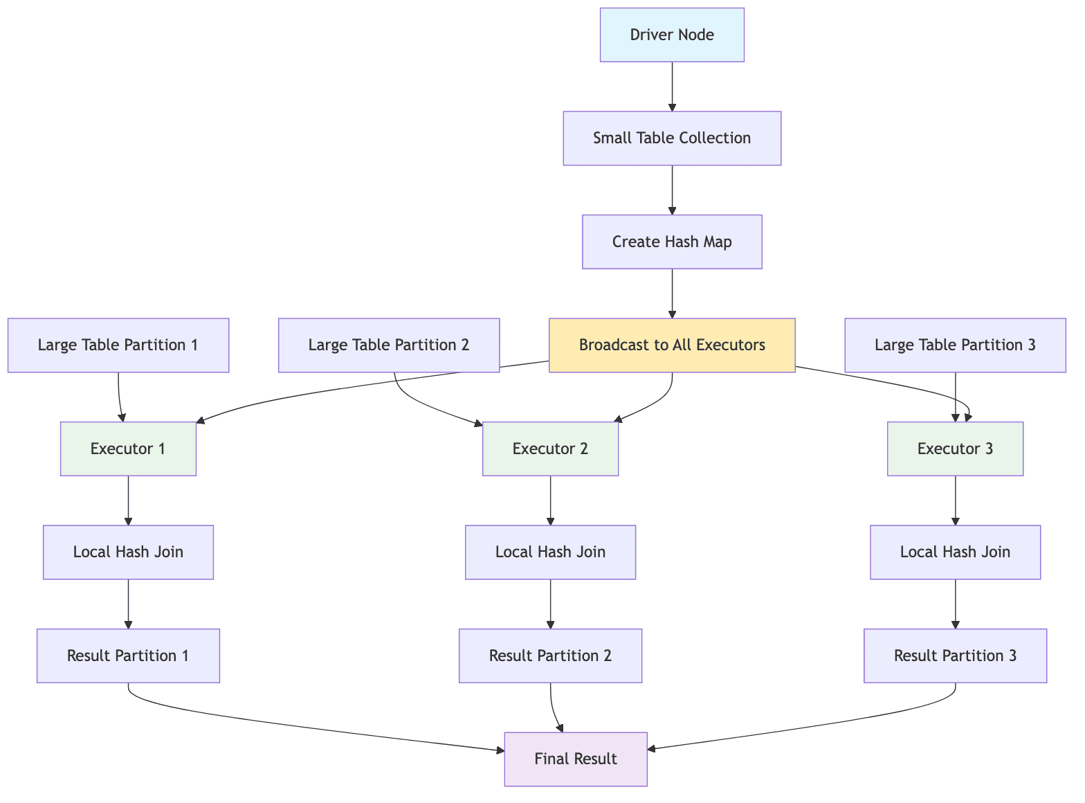
Broadcast Hash Join (BHJ)

The Broadcast Hash Join is Spark's most efficient join strategy when applicable. It follows the following process:

• The smaller of the two tables is collected entirely on the driver node
• The driver broadcasts this table as a read-only hash map to every executor node in the cluster
• Each executor that holds the partitions of the larger table performs a local hash join by iterating over its local rows and probing the in-memory broadcasted hash map for matches. The larger table is never shuffled across the network.

Spark's optimizer will automatically choose a BHJ when one of the tables is smaller than the configurable threshold: spark.sql.autoBroadcastJoinThreshold (default 10 MB). This strategy is ideal for star-schema joins where a large fact table is joined with much smaller dimension tables.

It is extremely fast as it completely avoids shuffling the larger table. However, the broadcast operation is itself network intensive and can become a bottleneck if the smaller table is moderately sized. More critically, if the smaller table exceeds the driver's available memory, it can cause an OutOfMemoryError (OOM) on the driver, crashing the entire job.

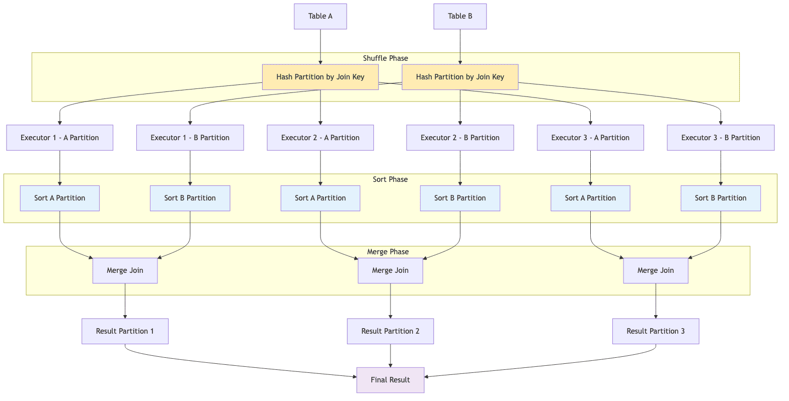
Shuffle Sort-Merge Join (SMJ)

When both tables are too large to broadcast, Spark's default strategy is the Shuffle Sort-Merge Join. It is a robust, multi-phase algorithm:

1. Shuffle Phase: Both tables are repartitioned across the cluster. Spark applies a hash function to the join key of each row to determine which executor the row should be sent to. This ensures that all rows with the same join key end up on the same executor for both tables.
2. Sort Phase: On each executor, the received data for each table is sorted by the join key within its partition. This sorting is crucial for the next phase. If the data for a partition doesn't fit in memory, Spark's external sort mechanism will spill intermediate data to disk and continue sorting.
3. Merge Phase: With both partitions on a worker now sorted by the join key, the join can be performed very efficiently. The engine iterates through both sorted datasets with two pointers, similar to the merge step of the classic merge-sort algorithm, and outputs the joined rows when the keys match.

SMJ is the default and the most common join strategy for joining two large tables.
It is highly scalable and memory-safe due to its ability to spill sorted runs to disk. It is also robust to data skew as the shuffle phase redistributes data evenly across executors (especially when combined with Adaptive Query Execution AQE). However, it is computationally intensive due to the sorting step and incurs significant network I/O during the shuffle phase.

Shuffle Hash Join (SHJ)

The Shuffle Hash Join offers a middle ground between BHJ and SMJ. It begins with the same shuffle phase as SMJ, where both tables are repartitioned across the cluster based on the join key. However, it bypasses the expensive sort phase. Instead, each executor takes the smaller of the two received partitions and builds an in-memory hash table on the join key. It then streams rows from the larger partition, probing the hash table for matches.

Spark may choose SHJ over SMJ when it determines that one of the shuffled partitions on each worker will be small enough to comfortably fit in memory as a hash table. This can be explicitly configured using the spark.sql.join.preferSortMergeJoin to false.

It can be significantly faster than SMJ because it avoids the expensive sort phase. However, it is susceptible to memory pressure. The hash table for the smaller partition must fit entirely within the executor's memory. If it exceeds available memory, it can lead to OOM errors on the executor, causing task failures and job retries.

Join Execution and Optimization in Trino

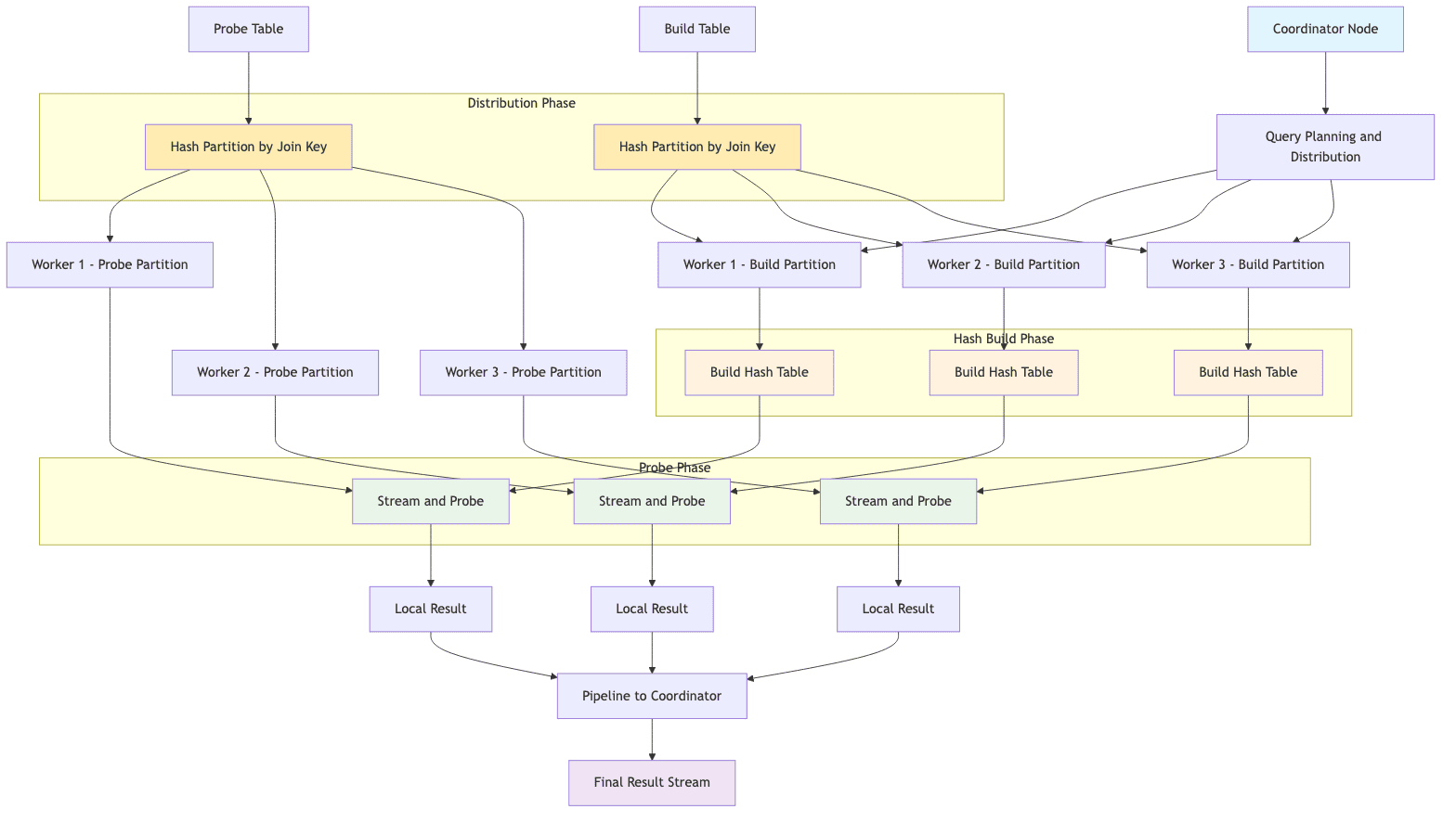
Trino's approach to join execution, as discussed, is tightly coupled with its MPP architecture and pipelined execution model.
It's architecture is that of a classic coordinator-worker MPP system. Trino relies exclusively on hash-based join algorithms. The primary decision its optimizer makes is how to distribute the data across the workers to perform the hash join efficiently.

Since Trino only uses hash-based joins, it always has build and probe phases. The engine consumes the entire build-side table and uses it to construct a hash table in the memory of the worker node. Once the hash table is complete, the probe side table is streamed through, row by row. For each row from the probe side, its join key is hashed and used to look up matching rows in the in-memory hash table. If matches are found, the joined rows are output. The key to performance is ensuring that the build side is smaller of the two tables and that the hash table can be built efficiently in memory.

Join Algorithms in Trino

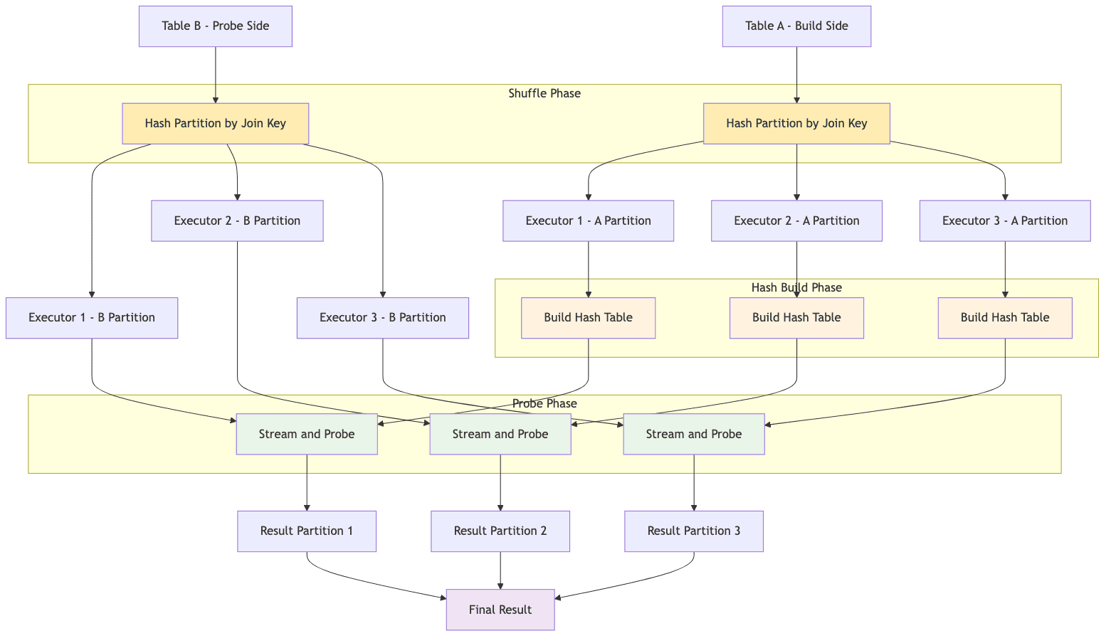
Partitioned Join

A partitioned join (also called a distributed join) is the default join strategy in Trino. It is used for handling joins between two large tables. In this mode, the build-side and the probe-side tables are repartitioned across the worker nodes. A hash function is applied to the join key of each row and rows are sent over the network to the worker responsible for that hash value. The result is that each worker receives a distinct slice or partition of both tables. Each worker then independently builds a hash table from its local partition of the build side and probes it with the corresponding partition of the probe side. This process is similar to the Shuffle Hash Join in Spark.

However, the sum of all hash tables across all workers must fit in the aggregate memory of the cluster.

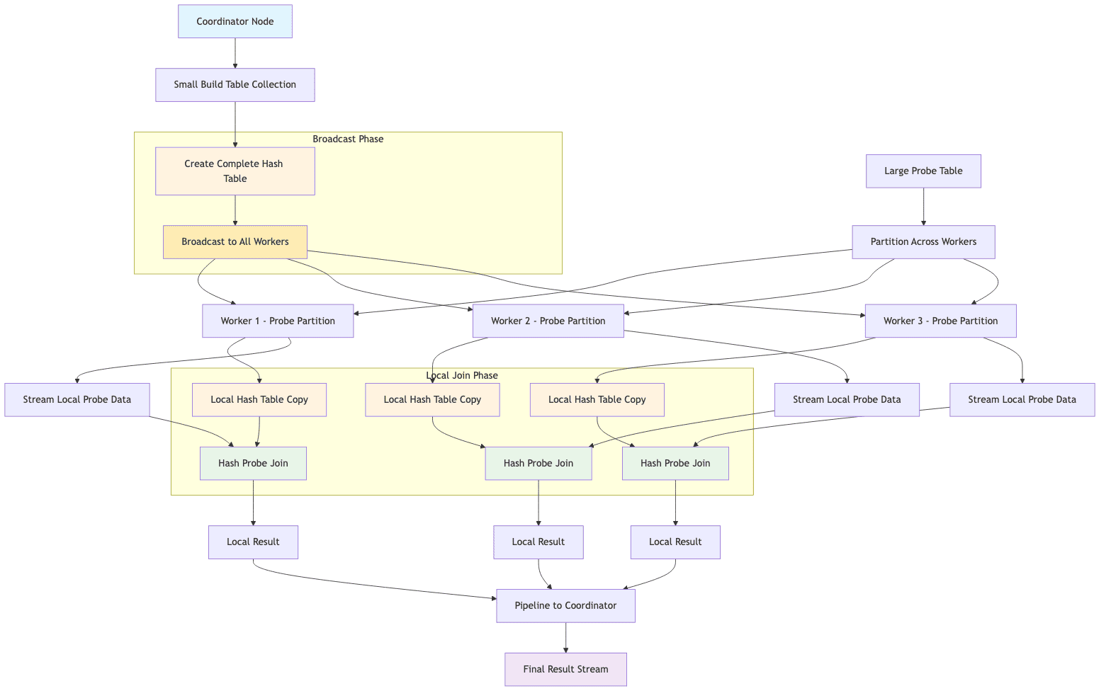
Broadcast Join

This join is analogous to Spark's Broadcast Hash Join and is used for asymmetric joins. The entire build-side table is replicated and sent to every worker node that holds at least one partition of the probe-side table. Each of these workers then builds a complete copy of the build-side hash table in its local memory. It then performs a local join by streaming its local partitions of the probe table against this hash table. It avoids costly network operation of hashing and repartitioning the much larger probe table.

Like the BHJ in Spark, this strategy is chosen when the build side table is small enough to fit comfortably in memory of each individual worker node. It is significantly faster than a partitioned join in these scenarios due to the elimination of the shuffle phase.

Cost-Based Optimizer (CBO)

Trino's coordinator houses a sophisticated Cost-based optimizer (CBO). When the join_distribution_type is set to AUTOMATIC, the CBO analyzes the table statistics (row counts, data sizes, cardinality etc.) provided by the underlying data source connectors. Based on these statistics, it estimates the computational and network costs for both partitioned and broadcast distribution strategies. It will automatically select the smaller table as the build side and decide whether to use broadcast or partitioned join. If statistics are unavailable, it defaults to a partitioned join.

Implementing Join Algorithms in Python

We'll now implement the various join algorithms discussed above in Python. The implementations will be simplified versions to illustrate the core concepts. The implementations only support inner-joins for simplicity. They do not handle all edge cases or optimizations present in production systems. Other types of joins (left, right, outer etc.) can be implemented similarly by adjusting the logic to handle non-matching rows appropriately.

Hash Join

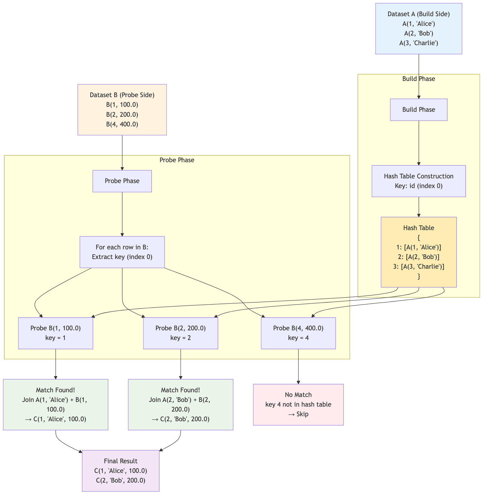
The Hash Join algorithm is a fundamental join strategy that operates in two distinct phases: build and probe. It is the foundation for more complex distributed join strategies like Spark's Broadcast Hash Join and Shuffle Hash Join.
Here's how it works with a concrete example:

Implementation Details

1# main hash join method
2def join(
3        self,
4        dataset1: BaseDataset[T],
5        dataset2: BaseDataset[U],
6        build_key_idx: int,
7        probe_key_idx: int,
8) -> BaseDataset[V]:
9    self.hash_table.clear()
10    # build phase
11    for row in dataset1:
12        key = astuple(row)[build_key_idx]
13        self.hash_table[key].append(row)
14
15    # probe phase
16    joined_rows = []
17    for row in dataset2:
18        key = astuple(row)[probe_key_idx]
19        if key in self.hash_table:
20            for match_row in self.hash_table[key]:
21                combined_tuple = self._combine_rows(match_row, row, probe_key_idx)
22                result_obj = self._create_result_object(combined_tuple)
23                joined_rows.append(result_obj)
24
25    return BaseDataset[V](rows=joined_rows)
26

The hash join algorithm follows these key steps:

1. Build Phase:

   • Iterate through the smaller dataset (Dataset A in our example)
   • Extract the join key from each row using build_key_idx
   • Store each row in a hash table using the join key
   • Multiple rows can have the same key (stored in a list)

2. Probe Phase:

   • Iterate through the larger dataset (Dataset B)
   • Extract the join key using probe_key_idx
   • Look up the key in the hash table
   • For each match found, combine the rows to create the result

Time Complexity Analysis

• Build Phase: O(n) where n is the size of the build-side dataset
• Probe Phase: O(m) where m is the size of the probe-side dataset
• Overall: O(n + m) - linear time complexity
• Space Complexity: O(n) for storing the hash table

Sort-Merge Join

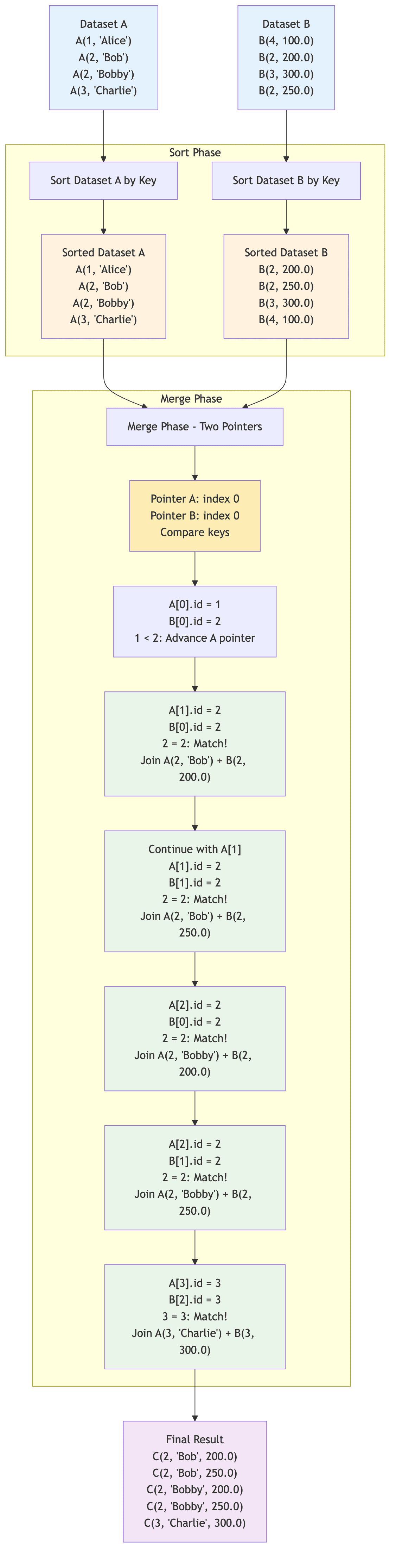
The Sort-Merge Join algorithm is a classic join strategy that is particularly effective for large datasets that do not fit into memory. It operates in three main phases: sort, merge, and join. This algorithm is the backbone of Spark's Shuffle Sort-Merge Join.

Implementation Details

1def join(
2    self,
3    dataset1: BaseDataset[T],
4    dataset2: BaseDataset[U],
5    build_key_idx: int,
6    probe_key_idx: int,
7) -> BaseDataset[V]:
8    # sort phase
9    sorted_dataset1 = sorted(dataset1, key=lambda row: astuple(row)[build_key_idx])
10    sorted_dataset2 = sorted(dataset2, key=lambda row: astuple(row)[probe_key_idx])
11
12    # merge phase
13    i, j = 0, 0
14    joined_rows = []
15
16    while i < len(sorted_dataset1) and j < len(sorted_dataset2):
17        row1 = sorted_dataset1[i]
18        row2 = sorted_dataset2[j]
19        key1 = astuple(row1)[build_key_idx]
20        key2 = astuple(row2)[probe_key_idx]
21
22        if key1 < key2:
23            i += 1
24        elif key1 > key2:
25            j += 1
26        else:
27            current_key = key1
28
29            # get all matching rows in dataset1 and dataset2
30            i_start = i
31            j_start = j
32
33            while (
34                i < len(sorted_dataset1)
35                and astuple(sorted_dataset1[i])[build_key_idx] == current_key
36            ):
37                i += 1
38
39            while (
40                j < len(sorted_dataset2)
41                and astuple(sorted_dataset2[j])[probe_key_idx] == current_key
42            ):
43                j += 1
44
45            i_end = i
46            j_end = j
47
48            # cartesian
49            for row1_idx in range(i_start, i_end):
50                for row2_idx in range(j_start, j_end):
51                    row1 = sorted_dataset1[row1_idx]
52                    row2 = sorted_dataset2[row2_idx]
53
54                    combined_tuple = self._combine_rows(row1, row2, probe_key_idx)
55                    result_obj = self._create_result_object(combined_tuple)
56                    joined_rows.append(result_obj)
57
58    return BaseDataset[V](rows=joined_rows)
59

The sort-merge join algorithm follows these key phases:

1. Sort Phase:

   • Both datasets are sorted by their respective join keys
   • Dataset A: Sorted by build_key_idx (id field)
   • Dataset B: Sorted by probe_key_idx (id field)
   • Time Complexity: O(n log n + m log m)

2. Merge Phase:

   • Use two pointers to traverse both sorted datasets
   • Compare join keys at current pointer positions
   • Advance pointers based on comparison results
   • When keys match, perform the join operation

The merge algorithm handles duplicate keys efficiently:

• Key Comparison: If A_key < B_key, advance A pointer
• Key Comparison: If A_key > B_key, advance B pointer
• Key Match: If A_key = B_key, join all combinations of matching rows
• Multiple Matches: Handle cases where both datasets have duplicate keys (like key=2 in our example)

External Sort-Merge Join

When datasets are too large to fit into memory, an external sort-merge join can be implemented. This involves breaking the datasets into smaller chunks that can be sorted in memory, writing these sorted chunks to disk, and then merging them in a way similar to the in-memory sort-merge join. You can find an example in the source code repository.

Time Complexity Analysis

• Sort Phase: O(n log n + m log m) for sorting both datasets
• Merge Phase: O(n + m) for single pass through sorted data
• Overall: O(n log n + m log m) - dominated by sorting
• Space Complexity: O(1) additional space (in-place merge)

Grace & Parallel Hash Joins

Grace Hash Join and Parallel Hash Join are advanced join strategies designed to handle very large datasets that exceed available memory. They extend the basic hash join algorithm by partitioning the data into smaller chunks that can be processed independently.

Grace Hash Join

The Grace Hash Join algorithm partitions both datasets into smaller buckets based on a hash function applied to the join key. Each bucket is small enough to fit into memory, allowing the hash join to be performed on each partition independently.

Grace Hash Join is optimal when:

• Datasets are too large to fit in memory for regular hash join
• You have sufficient disk space for temporary partitions
• Memory is limited but disk I/O is acceptable
• Data distribution allows for effective partitioning
• You need guaranteed completion regardless of data size

Implementation Details

1def join(
2        self,
3        dataset1: BaseDataset[T],
4        dataset2: BaseDataset[U],
5        build_key_idx: int,
6        probe_key_idx: int,
7) -> BaseDataset[V]:
8    partition_files1 = []
9    partition_files2 = []
10    if hasattr(self, "_type_params") and len(getattr(self, "_type_params")) >= 3:
11        params = getattr(self, "_type_params")
12        hash_joiner_class = HashJoinAlgorithm[params[0], params[1], params[2]]
13        hash_joiner = hash_joiner_class()
14    else:
15        hash_joiner = HashJoinAlgorithm()
16        hash_joiner._result_type = self._result_type
17
18    try:
19        partition_files1, partition_files2 = self._partition_datasets(
20            dataset1, dataset2, build_key_idx, probe_key_idx
21        )
22
23        joined_rows = []
24
25        for i in range(self.NUM_PARTITIONS):
26            partition_files1[i].seek(0)
27            partition_files2[i].seek(0)
28
29            # dangerous; only for demo purposes
30            build_side = [eval(row.strip()) for row in partition_files1[i]]
31            probe_side = [eval(row.strip()) for row in partition_files2[i]]
32
33            partial_joined = hash_joiner.join(
34                BaseDataset[T](rows=build_side),
35                BaseDataset[U](rows=probe_side),
36                build_key_idx,
37                probe_key_idx,
38            ).rows
39            joined_rows.extend(partial_joined)
40        return BaseDataset[V](rows=joined_rows)
41
42    finally:
43        for f in partition_files1 + partition_files2:
44            try:
45                f.close()
46                os.remove(f.name)
47            except Exception as e:
48                print(f"Error cleaning up file {f.name}: {e}")
49

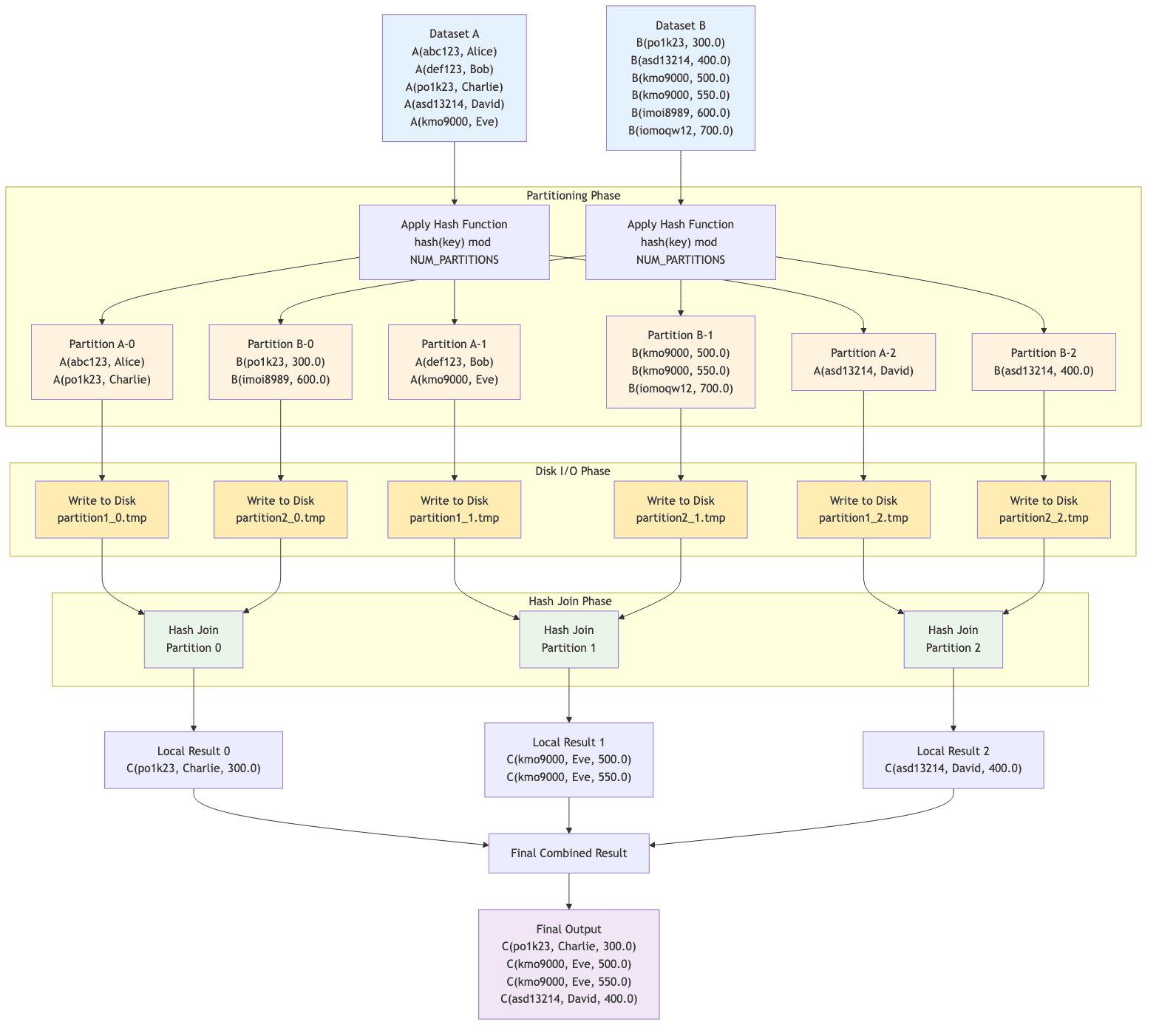
The Grace Hash Join algorithm operates in three distinct phases:

1. Partitioning Phase:

   • Apply hash function hash(key) % NUM_PARTITIONS to join keys
   • Partition both datasets into N buckets based on hash values
   • Ensures matching keys end up in the same partition number
   • Example: hash('po1k23') % 3 = 0 for both datasets

2. Disk I/O Phase:

   • Write each partition to temporary files on disk
   • Allows processing datasets larger than available memory
   • Files: partition1_0.tmp, partition1_1.tmp, etc.
   • Each partition should fit comfortably in memory

3. Hash Join Phase:

   • Load corresponding partitions from disk (one at a time)
   • Perform standard hash join on each partition pair
   • Combine results from all partitions
   • Clean up temporary files

Hash Function Distribution

In our example with NUM_PARTITIONS = 3:

Partition 0: Keys that hash to 0

• 'abc123' → Alice (no match in B)
• 'po1k23' → Charlie ↔ 300.0 ✓
• 'imoi8989' → 600.0 (no match in A)

Partition 1: Keys that hash to 1

• 'def123' → Bob (no match in B)
• 'kmo9000' → Eve ↔ 500.0, 550.0 ✓
• 'iomoqw12' → 700.0 (no match in A)

Partition 2: Keys that hash to 2

• 'asd13214' → David ↔ 400.0 ✓

Time Complexity Analysis

• Partitioning Phase: O(n + m) to read and hash partition both datasets
• I/O Phase: O(n + m) to write all data to disk
• Join Phase: O(n + m) total across all partitions
• Overall: O(n + m) - linear time complexity
• Space Complexity: O(max_partition_size) in memory + O(n + m) on disk

Parallel Hash Join

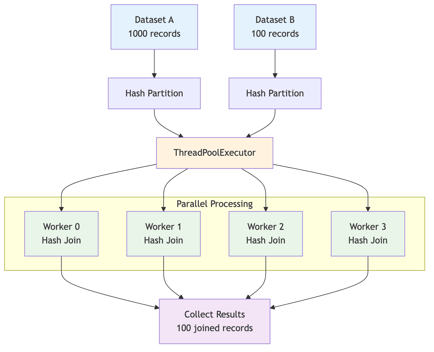
Parallel Hash Join uses concurrent processing to perform hash joins on multiple partitions simultaneously. This approach is particularly effective in distributed systems where multiple processors or nodes can work in parallel. In our example in the repository, we simulate parallelism using Python's concurrent.futures module to run hash joins on different partitions concurrently.

Parallel Hash Join is optimal when:

• Multiple CPU cores or processors are available
• Datasets can be effectively partitioned by hash function
• Memory per worker is sufficient for local hash tables
• Network overhead is minimal (in distributed scenarios)
• Maximize throughput for large-scale joins

Implementation Details

1def join(
2    self,
3    dataset1: BaseDataset[T],
4    dataset2: BaseDataset[U],
5    build_key_idx: int,
6    probe_key_idx: int,
7) -> BaseDataset[V]:
8    joined_rows = []
9
10    with ThreadPoolExecutor(max_workers=self.NUM_WORKERS) as executor:
11        futures = [
12            executor.submit(
13                self._worker_join,
14                worker_id,
15                dataset1,
16                dataset2,
17                build_key_idx,
18                probe_key_idx,
19            )
20            for worker_id in range(self.NUM_WORKERS)
21        ]
22        for future in as_completed(futures):
23            try:
24                worker_result = future.result()
25                joined_rows.extend(worker_result.rows)
26            except Exception as e:
27                print(f"Worker encountered an error: {e}")
28                raise
29
30    print("Sample joined rows:")
31    print("\n".join(map(str, joined_rows[:10])))
32    return BaseDataset[V](rows=joined_rows)
33

The Parallel Hash Join algorithm operates in three main phases:

1. Partitioning Phase:

   • Apply hash function hash(key) % NUM_WORKERS to both datasets
   • Distribute records across worker partitions based on hash values
   • Ensures matching keys end up in the same worker partition
   • Each worker gets roughly equal data distribution

2. Parallel Execution Phase:

   • Launch multiple worker threads using ThreadPoolExecutor
   • Each worker processes its assigned partition independently
   • Workers perform standard hash join on their local partitions
   • All workers execute concurrently for maximum throughput

3. Result Aggregation Phase:

   • Collect results from all workers using as_completed
   • Combine partial results into final dataset
   • Handle any worker exceptions gracefully

Data Distribution

With 4 workers processing the example data:

Dataset A (1000 records): A(1, name_1) through A(1000, name_1000)

• Worker 0: Records with hash(id) % 4 = 0 (~250 records)
• Worker 1: Records with hash(id) % 4 = 1 (~250 records)
• Worker 2: Records with hash(id) % 4 = 2 (~250 records)
• Worker 3: Records with hash(id) % 4 = 3 (~250 records)

Dataset B (100 records): B(500, 750.0) through B(599, 898.5)

• Each worker gets ~25 records from the overlapping range
• Only records with matching hash values will be in same worker

Performance Characteristics

• Time Complexity: O((n + m) / p) where p is number of workers
• Space Complexity: O(max_partition_size) per worker
• Scalability: Linear speedup with available CPU cores
• Memory Usage: Distributed across workers, reduces peak memory

Conclusion

In this article, we explored the join algorithms employed by distributed query engines like Apache Spark and Trino. We examined how their architectural choices influence their join strategies, with Spark prioritizing fault tolerance and scalability through the Shuffle Sort-Merge Join, while Trino focuses on low-latency performance with hash-based joins.

We also implemented simplified versions of these join algorithms in Python, including Hash Join, Sort-Merge Join, Grace Hash Join and Parallel Hash Join. These implementations illustrate the core concepts and trade-offs involved in each strategy.

If you have any questions, corrections, feedback or suggestions, please reach out! I'd love to hear your thoughts.