Contextual Bandits for Marketing

It's been a while since I last got my hands dirty with some ML topics. I recently came across the use of contextual bandits in marketing strategies and found it interesting enough to explore further. While I'm no expert in this topic, I wanted to delve into it and share my findings with you.

Contextual bandits are a type of ML(reinforcement learning) algorithms that can be used to optimize marketing strategies by learning from user interactions. They are particularly useful in scenarios where you want to personalize content or offers based on user characteristics and behaviors.

In this post, we will explore how to implement some contextual bandit algorithms using Python and run them on a simulated marketing dataset. We will also go over how these algorithms can be deployed in production and monitored for performance.

🔗 Source Code: abyssnlp/contextual-bandits

---

Contents

1. Introduction to Multi-armed Bandits
2. Contextual Bandits
3. Types of Contextual Bandit Algorithms
   1. LinUCB (Linear Upper Confidence Bound)
      1. LinUCB Score
      2. Parameter Updates
      3. Intuition
   2. Neural Bandits
      1. How it works
      2. Difference from LinUCB
   3. Production Considerations
      1. Data size and training
      2. Computational cost
      3. Monitoring and debugging
      4. Expertise
4. Simulating Contextual bandits on synthetic marketing data
   1. Generating synthetic marketing data
   2. Running the simulation
5. Architecture for Production
   1. Model deployment
   2. Online feature serving
   3. Request Response logging
   4. Writing to the offline store
   5. Retraining the model
   6. Model registry
   7. Observability
   8. Security & Compliance
6. Conclusion

Introduction to Multi-armed Bandits

Multi-armed bandits (MAB) are a class of problems in reinforcement learning where an agent must choose between multiple options (or "arms" or "actions") to maximize some reward. The classic example is a slot machine with multiple levers, where each lever has a different probability of winning. The goal is to find the best lever to pull to maximize the total reward. The challenge is to balance two polar objectives:

• Exploration: Trying different actions/arms to gather information about their rewards
• Exploitation: Choosing the action/arm that has the highest expected reward based on the information gathered so far

An easier example is a website with multiple versions of a landing page, where each version has a different conversion rate. MAB could be used to determine as well as personalize which version of the landing page to show to each user based on their characteristics and behaviors.

In the world of marketing, MAB can be used to optimize various strategies such as email campaigns, ad placements and content recommendations. The key is to learn from the user interactions and update the strategy accordingly to maximize the reward (ex. click-through rate, conversion rate, etc.).

Contextual Bandits

Traditional multi-armed bandits assume that the reward for each action is static. However, real world scenarios often involve contextual information that can influence optimal decisions. Contextual bandits extend the MAB framework by incorporating additional information (context) about the user or the environment when making decisions. This allows for more personalized and effective strategies.

For example, in marketing, the context could include user demographics, events, past interactions or any other relevant information that can help predict the reward for each action. By using this context, contextual bandits tailor strategies to individual users, leading to better performance in highly dynamic environments.

In contextual bandits, at each time step:

1. The agent observes the context vector x_t which contains information about the user or the environment.
2. The agent selects an arm/action a_t based on the context and its current policy.
3. The agent receives a reward r_t based on the action taken and the context.
4. The agent updates its policy based on the observed reward and context.

The process continues iteratively so the agent learns to optimize its actions over time.

In a marketing context, the context might include:

• User features: demographics, preferences, past behaviors
• Content/Item features: Content category, popularity, price
• Temporal features: Time of the day, season
  and so on.

Types of Contextual Bandit Algorithms

There are several algorithms for contextual bandits, each with their own strengths and weaknesses. We'll be discussing 2 of the most popular ones:

1. LinUCB (Linear Upper Confidence Bound)
2. Neural Bandits

LinUCB (Linear Upper Confidence Bound)

LinUCB uses linear regression to model the relationship between the context and the expected reward. It maintains a set of parameters that are updated based on the observed rewards. It balances exploration and exploitation by using an upper confidence bound on the expected reward.

It maintains:

• A weight vector estimating reward parameters for each arm
• A covariance matrix to capture uncertainty in the estimates

Suppose at each round $t$, we have a set of arms (actions), each with a context (feature) vector $x_{a,t} \in \mathbb{R}^d$. The expected reward for arm $a$ is assumed to be linear in the context:

$\mathbb{E}[r_{a,t} \mid x_{a,t}] = x_{a,t}^\top \theta^*$

where $\theta^* \in \mathbb{R}^d$ is an unknown parameter vector.

LinUCB Score

For each arm $a$, LinUCB computes an upper confidence bound:

$\text{UCB}_{a,t} = x_{a,t}^\top \hat{\theta}_t + \alpha \cdot \sqrt{x_{a,t}^\top A_t^{-1} x_{a,t}}$

• $\hat{\theta}_t$ is the ridge regression estimate of $\theta^*$ at time $t$
• $A_t = D_t^\top D_t + \lambda I$, where $D_t$ is the matrix of observed context vectors up to time $t$, and $\lambda$ is a regularization parameter
• $\alpha > 0$ controls the width of the confidence interval (exploration parameter)
• The first term is the estimated reward; the second term quantifies uncertainty

Parameter Updates

After selecting arm $a_t$ and observing reward $r_{a_t, t}$:

Update covariance matrix that tracks feature correlations:
$A_t \leftarrow A_{t-1} + x_{a_t, t} x_{a_t, t}^\top$

Update reward vector:
$b_t \leftarrow b_{t-1} + r_{a_t, t} x_{a_t, t}$

Compute the updated parameter estimate:
$\hat{\theta}_t = A_t^{-1} b_t$

Intuition

• Exploitation: The algorithm prefers arms with high estimated reward ($x_{a,t}^\top \hat{\theta}_t$).
• Exploration: The uncertainty term ($\sqrt{x_{a,t}^\top A_t^{-1} x_{a,t}}$) encourages trying arms with less data.
• Balance: The parameter $\alpha$ tunes the trade-off between exploration and exploitation.

The mathematics for this is more daunting than the actual implemention in code using numpy. Each line in the above equations corresponds to a line in the code below.

1for arm in range(self.n_arms):
2    A_inv = np.linalg.solve(self.A[arm], np.eye(self.context_dim))
3    self.theta[arm] = A_inv @ self.b[arm]
4    expected_reward = context.dot(self.theta[arm])
5    cb = self.alpha * np.sqrt(context.dot(A_inv).dot(context))
6    ucb_values[arm] = expected_reward + cb
7
8best_arm = np.argmax(ucb_values)
9

Neural Bandits

Neural bandits extend the contextual bandit framework by using neural networks to model the relationship between context and expected reward. Unlike linear methods like LinUCB, neural bandits assumes that the relationship between the context and the reward is non-linear and complex.

It uses the representational power of neural networks to learn this relationship from the data.

How it works

The neural bandit algorithm I've implemented maintains a separate neural network for each arm, where each network learns to predict the expected reward given the context. The architecture consists of fully connected layers with ReLU(Rectified Linear Unit) activations. The output layer has a single neuron that predicts the expected reward. This allows it to capture complex non-linear relationships.

1layers = []
2input_dim = context_dim
3
4for dim in hidden_dims:
5    layers.append(nn.Linear(input_dim, dim))
6    layers.append(nn.ReLU())
7    input_dim = dim
8
9layers.append(nn.Linear(input_dim, 1))
10self.network = nn.Sequential(*layers)
11

The implementation also follows an epsilon-greedy strategy for exploration. With probability epsilon, it selects a random arm to explore. Otherwise, with probability 1 - epsilon, it selects the arm with the highest predicted reward from the neural networks.

1# epsilon-greedy exploration
2if np.random.random() < self.epsilon:
3    return np.random.randint(self.n_arms)
4
5# else, select the arm with the highest predicted reward
6

Difference from LinUCB

• LinUCB assumes a linear relationship between the context and the expected reward, while neural bandits can capture more complex, non-linear relationships.

• LinUCB maintains confidence intervals around reward estimates and selects arms based on upper confidence bounds, providing a principled exploration-exploitation trade-off. Neural bandits on the other hand, rely on epsilon-greedy exploration.

• LinUCB comes with proven regret bounds and theoretical guarantees, while neural bandits are more empirical and require hyperparameter tuning and large amount of data to perform well.

Production Considerations

Data size and training

Neural bandits typically require larger datasets to train effectively compared to linear models like LinUCB. In my implementation, it accumulates data until reaching batch_size before training, which can lead to poor early performance if the data is sparse. Linear methods like LinUCB can start making reasonable decisions with much less data, updating incrementally with each observation.

Computational cost

Neural bandits require GPU resources for training, especially with larger networks for more epochs. This can be a bottleneck in production environments, especially if real-time decisions are needed. LinUCB is computationally efficient, requiring only matrix operations that can be performed on the CPU.

Monitoring and debugging

Neural bandits can be harder to monitor and debug due to their complexity. They need careful monitoring of training loss, validation performance and hyperparameter tuning. LinUCB is more interpretable and easier to monitor and debug with more predictable behavior.

Expertise

Neural bandits require expertise in deep learning and neural network architectures, which may not be available in all teams. LinUCB is simpler and requires less specialized knowledge, making it more accessible for teams with limited ML expertise.

Simulating Contextual bandits on synthetic marketing data

Generating synthetic marketing data

To demonstrate their usage, I created a synthetic dataset that simulates a user context and their interactions with different email campaigns. It contains features like user demographics, past purchases, email engagement and temporal metrics like hour of day and day of the week.

The simple function to generate synthetic marketing data can be found under /examples/generate_data.py. It outputs a pandas DataFrame with n_samples rows.

1def generate_marketing_data(
2    n_samples: int = 1000,
3    n_campaigns: int = 5,
4    n_user_features: int = 10,
5    random_state: t.Optional[int] = None,
6) -> pd.DataFrame:
7    if random_state is not None:
8        np.random.seed(random_state)
9
10    user_features = np.random.randn(n_samples, n_user_features)
11    campaigns = np.random.randint(0, n_campaigns, size=n_samples)
12    campaign_params = np.random.randn(n_campaigns, n_user_features)
13    conversion_probs = np.zeros(n_samples)
14    for i in range(n_samples):
15        logit = np.dot(user_features[i], campaign_params[campaigns[i]])
16        conversion_probs[i] = 1.0 / (1.0 + np.exp(-logit))
17
18    conversions = np.random.binomial(1, conversion_probs)
19    unsubscribe_probs = 0.01 + 0.1 * (1 - conversion_probs)
20    unsubscribes = np.random.binomial(1, unsubscribe_probs)
21
22    df = pd.DataFrame()
23    for i in range(n_user_features):
24        df[f"user_feature_{i}"] = user_features[:, i]
25    df["age_group"] = np.random.choice(
26        ["18-24", "25-34", "35-44", "45-54", "55+"], size=n_samples
27    )
28    df["gender"] = np.random.choice(["M", "F", "Other"], size=n_samples)
29    df["device"] = np.random.choice(["Mobile", "Desktop", "Tablet"], size=n_samples)
30    df["previous_purchases"] = np.random.poisson(2, size=n_samples)
31    df["campaign_id"] = [f"campaign_{c}" for c in campaigns]
32    df["email_opened"] = np.random.binomial(1, 0.3 + 0.4 * conversion_probs)
33    df["email_clicked"] = (
34        np.random.binomial(1, 0.2 + 0.6 * conversion_probs)
35        * df["email_opened"]  # only clicked if opened
36    )
37    df["conversion"] = conversions
38    df["unsubscribe"] = unsubscribes
39    df["day_of_week"] = np.random.randint(0, 7, size=n_samples)
40    df["hour_of_day"] = np.random.randint(0, 24, size=n_samples)
41
42    return df
43

Running the simulation

We'll now run the simulation against this synthetic marketing dataset using both LinUCB and Neural bandits. We'll also use a random policy as baseline for comparison.

For creating one-off scripts, I find using AI tools like Claude to be very helpful. The run_simulation.py script is generated using Claude, which takes the synthetic dataset and runs the simulation for each of the three algorithms.

The BanditSimulation class orchestrates the simulation starting with synthetic data generation. This data is then split into training and test sets. It avoids data leakage by ensuring that the test set is not used for training the bandit algorithms.

During the online phase, each algorithm observes a user context and selects a campaign to show. The algorithm then receives a reward based on the user's interaction with the email camapaign. The algorithms only observer rewards for the campaigns they selected and not counterfactual rewards for campaigns they did not select. The simulation tracks the cumulative rewards and regret (the difference between the reward of the best campaign and the selected campaign) over time.

At the end, the simulation visualizes the cumulative rewards and regret for each algorithm, for each campaign(arm).

Something to note is that we're using discrete rewards (0 or 1) for conversions/clicks. This is a simplification, but in practice, you might want to use continuous rewards based on the value of the conversion (e.g. revenue generated).

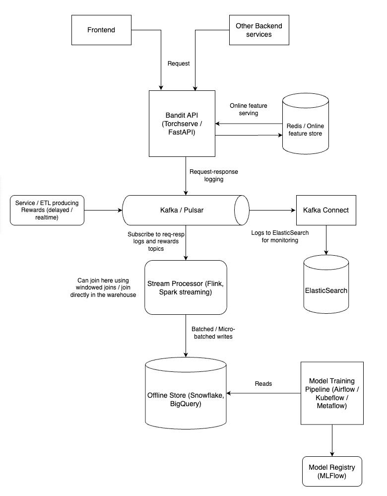
Architecture for Production

Contextual bandits like any other ML model need good MLOps practices to be deployed in production.

Model deployment

The model deployment would include using a model serving framework like TorchServe or FastAPI to serve the trained models. The model server would expose an API endpoint that can be called either from the frontend or any other backend service to get the recommended campaign for a user based on their context.

Online feature serving

The deployed model would need access to fresh user context features. This can be achieved using a feature store like Feast or a custom feature serving solution can also be rolled out. The online feature serving system would provide updated user context features to the model server in real-time. It should be updated frequently by backend services that collect user information and interactions. Ideally, this should be updated using a message/event bus like Kafka or Pulsar to ensure non-blocking low-latency and high-throughput updates.

Request Response logging

To monitor the performance of the deployed model, we need to log the requests and responses. This includes logging the user context, the selected campaign, the observed reward and any other relevant information. There are several ways this can be accomplished. I recommend producing the logs to a message bus like Kafka/Pulsar. This allows these logs to be consumed downstream by multiple systems for different purposes like monitoring, analytics, etc.
These logs should be stored in the message bus with a request ID/correlation ID so we can join them with the rewards later.

Writing to the offline store

The logged requests and responses should be written to an offline store for further analysis. This can be done using a data warehouse like Snowflake or Bigquery, or a data like on S3.
The data here can be joined with the rewards data (for ex. in an email campaign, the rewards are usually delayed i.e. the user might not convert immediately after receiving the email) to create a complete dataset for offline analysis and retraining.

Retraining the model

After the above step, we should have a complete dataset for retraining our model in the data warehouse/ data lake. To retrain the model, we can use an orchestration tool like Airflow or ML pipeline tools like Kubeflow or Metaflow. These tools can be used to schedule and run the retraining jobs periodically or based on certain trigger (eg. model or data drift).

Model registry

The retrained model should be registered in a model registry like MLflow or Seldon. This allows us to keep track of the different versions of the model and their performance. The model registry can also be used to deploy the new model version to production.

Deployments can be done using a canary or blue-green deployment strategy. Model artefacts can be pulled on pod startup from the model registry. To fintetune deployments, we can use tools like Argo rollouts.

Observability

We can produce metrics to monitoring systems like Prometheus and visualize them on Grafana to monitor the performance of the deployed model. This includes metrics like:

• Cumulative rewards
• Regret
• inference latency
• exploration vs exploitation ratio
• per-arm CTR (Click Through Rate)
• per-arm conversion rate

Ofcourse, some of these metrics will differ based on the type of problem you're solving. For example, in an email campaign, the rewards are usually delayed i.e. the user might not convert immediately after receiving the email. In such cases, we can use a delayed reward metric to monitor the performance of the model on the analytics side.

Security & Compliance

We can hash PII data before producing it to the message bus to ensure that we are not storing any PII data in the logs. We can also use encryption to secure the data in transit and at rest.
On the data lake side, we can archive the data periodically to reduce storage costs and ensure compliance with data retention policies.

Conclusion

Contextual bandits are a powerful tool for optimizing marketing strategies by learning from user interactions. They allow for personalized content and offers based on user characteristics and behaviors. In this post, we explored how to implement LinUCB and Neural bandits using Python and run them on a simulated marketing dataset. We also discussed the production considerations for deploying these algorithms in real-world scenarios.

I hope this post has given you a good introduction to contextual bandits and how they can be run in production for use cases like optimising marketing strategies. If you have any questions, feedback, corrections or suggestions, please feel free to leave a comment down below. I'd love to hear your thoughts and experiences with contextual bandits or any other related topics.